
Note
Go to the end to download the full example code.
Isentropic Analysis#
The MetPy function mpcalc.isentropic_interpolation allows for isentropic analysis from model analysis data in isobaric coordinates.
import cartopy.crs as ccrs
import cartopy.feature as cfeature
import matplotlib.pyplot as plt
import numpy as np
import xarray as xr

import metpy.calc as mpcalc
from metpy.cbook import get_test_data
from metpy.plots import add_metpy_logo, add_timestamp
from metpy.units import units
Getting the data
In this example, [NARR reanalysis data]( https://www.ncei.noaa.gov/products/weather-climate-models/north-american-regional) for 18 UTC 04 April 1987 from the National Centers for Environmental Information will be used.
data = xr.open_dataset(get_test_data('narr_example.nc', False))
print(list(data.variables))
['Temperature', 'time', 'isobaric', 'y', 'x', 'Lambert_Conformal', 'lat', 'lon', 'u_wind', 'v_wind', 'Geopotential_height', 'Specific_humidity']
We will reduce the dimensionality of the data as it is pulled in to remove an empty time dimension, as well as add longitude and latitude as coordinates (instead of data variables).
data = data.squeeze().set_coords(['lon', 'lat'])
To properly interpolate to isentropic coordinates, the function must know the desired output isentropic levels. An array with these levels will be created below.
isentlevs = [296.] * units.kelvin
Conversion to Isentropic Coordinates
Once three dimensional data in isobaric coordinates has been pulled and the desired isentropic levels created, the conversion to isentropic coordinates can begin. Data will be passed to the function as below. The function requires that isentropic levels, as well as a DataArray of temperature on isobaric coordinates be input. Any additional inputs (in this case specific humidity, geopotential height, and u and v wind components) will be logarithmicaly interpolated to isentropic space.
isent_data = mpcalc.isentropic_interpolation_as_dataset(
    isentlevs,
    data['Temperature'],
    data['u_wind'],
    data['v_wind'],
    data['Specific_humidity'],
    data['Geopotential_height']
)
/home/runner/work/MetPy/MetPy/examples/isentropic_example.py:60: UserWarning: Interpolation point out of data bounds encountered
  isent_data = mpcalc.isentropic_interpolation_as_dataset(
The output is an xarray Dataset:
Note that the units on our wind variables are not ideal for plotting. Instead, let us convert them to more appropriate values.
isent_data['u_wind'] = isent_data['u_wind'].metpy.convert_units('kt')
isent_data['v_wind'] = isent_data['v_wind'].metpy.convert_units('kt')
Converting to Relative Humidity
The NARR only gives specific humidity on isobaric vertical levels, so relative humidity will have to be calculated after the interpolation to isentropic space.
isent_data['Relative_humidity'] = mpcalc.relative_humidity_from_specific_humidity(
    isent_data['pressure'],
    isent_data['temperature'],
    isent_data['Specific_humidity']
).metpy.convert_units('percent')
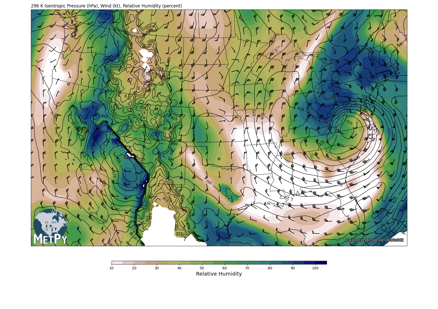
Plotting the Isentropic Analysis
# Set up our projection and coordinates
crs = ccrs.LambertConformal(central_longitude=-100.0, central_latitude=45.0)
lon = isent_data['pressure'].metpy.longitude
lat = isent_data['pressure'].metpy.latitude

# Coordinates to limit map area
bounds = [(-122., -75., 25., 50.)]
# Choose a level to plot, in this case 296 K (our sole level in this example)
level = 0

fig = plt.figure(figsize=(17., 12.))
add_metpy_logo(fig, 120, 245, size='large')
ax = fig.add_subplot(1, 1, 1, projection=crs)
ax.set_extent(*bounds, crs=ccrs.PlateCarree())
ax.add_feature(cfeature.COASTLINE.with_scale('50m'), linewidth=0.75)
ax.add_feature(cfeature.STATES, linewidth=0.5)

# Plot the surface
clevisent = np.arange(0, 1000, 25)
cs = ax.contour(lon, lat, isent_data['pressure'].isel(isentropic_level=level),
                clevisent, colors='k', linewidths=1.0, linestyles='solid',
                transform=ccrs.PlateCarree())
cs.clabel(fontsize=10, inline=1, inline_spacing=7, fmt='%i', rightside_up=True,
          use_clabeltext=True)

# Plot RH
cf = ax.contourf(lon, lat, isent_data['Relative_humidity'].isel(isentropic_level=level),
                 range(10, 106, 5), cmap=plt.cm.gist_earth_r, transform=ccrs.PlateCarree())
cb = fig.colorbar(cf, orientation='horizontal', aspect=65, shrink=0.5, pad=0.05,
                  extendrect='True')
cb.set_label('Relative Humidity', size='x-large')

# Plot wind barbs
ax.barbs(lon.values, lat.values, isent_data['u_wind'].isel(isentropic_level=level).values,
         isent_data['v_wind'].isel(isentropic_level=level).values, length=6,
         regrid_shape=20, transform=ccrs.PlateCarree())

# Make some titles
ax.set_title(f'{isentlevs[level]:~.0f} Isentropic Pressure (hPa), Wind (kt), '
             'Relative Humidity (percent)', loc='left')
add_timestamp(ax, isent_data['time'].values.astype('datetime64[ms]').astype('O'),
              y=0.02, high_contrast=True)
fig.tight_layout()
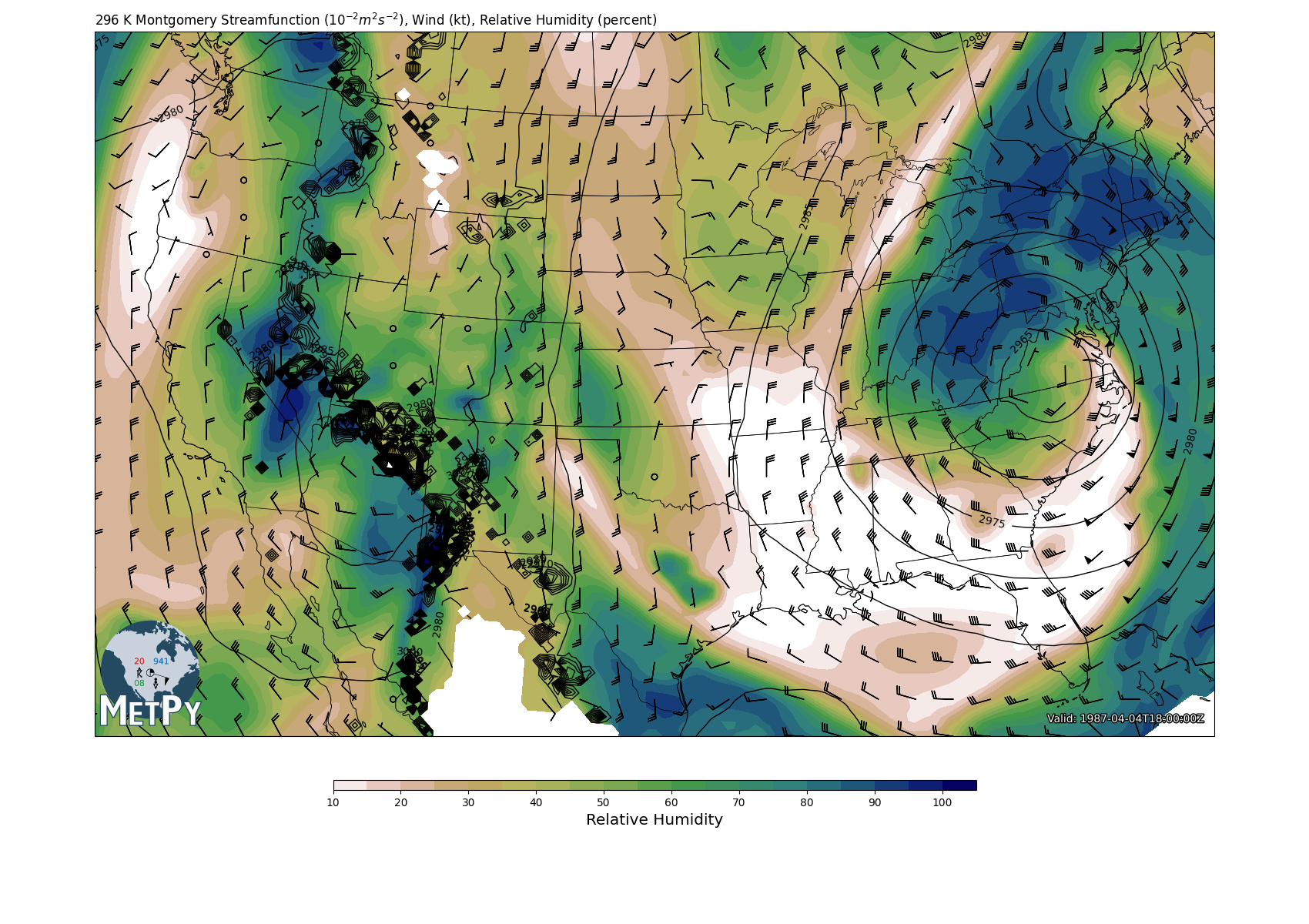
Montgomery Streamfunction
The Montgomery Streamfunction, \({\psi} = gdz + CpT\), is often desired because its gradient is proportional to the geostrophic wind in isentropic space. This can be easily calculated with mpcalc.montgomery_streamfunction.
# Calculate Montgomery Streamfunction and scale by 10^-2 for plotting
msf = mpcalc.montgomery_streamfunction(
    isent_data['Geopotential_height'],
    isent_data['temperature']
).data.to_base_units() * 1e-2

# Choose a level to plot, in this case 296 K
level = 0

fig = plt.figure(figsize=(17., 12.))
add_metpy_logo(fig, 120, 250, size='large')
ax = plt.subplot(111, projection=crs)
ax.set_extent(*bounds, crs=ccrs.PlateCarree())
ax.add_feature(cfeature.COASTLINE.with_scale('50m'), linewidth=0.75)
ax.add_feature(cfeature.STATES.with_scale('50m'), linewidth=0.5)

# Plot the surface
clevmsf = np.arange(0, 4000, 5)
cs = ax.contour(lon, lat, msf[level, :, :], clevmsf,
                colors='k', linewidths=1.0, linestyles='solid', transform=ccrs.PlateCarree())
cs.clabel(fontsize=10, inline=1, inline_spacing=7, fmt='%i', rightside_up=True,
          use_clabeltext=True)

# Plot RH
cf = ax.contourf(lon, lat, isent_data['Relative_humidity'].isel(isentropic_level=level),
                 range(10, 106, 5), cmap=plt.cm.gist_earth_r, transform=ccrs.PlateCarree())
cb = fig.colorbar(cf, orientation='horizontal', aspect=65, shrink=0.5, pad=0.05,
                  extendrect='True')
cb.set_label('Relative Humidity', size='x-large')

# Plot wind barbs
ax.barbs(lon.values, lat.values, isent_data['u_wind'].isel(isentropic_level=level).values,
         isent_data['v_wind'].isel(isentropic_level=level).values, length=6,
         regrid_shape=20, transform=ccrs.PlateCarree())

# Make some titles
ax.set_title(f'{isentlevs[level]:~.0f} Montgomery Streamfunction '
             r'($10^{-2} m^2 s^{-2}$), Wind (kt), Relative Humidity (percent)', loc='left')
add_timestamp(ax, isent_data['time'].values.astype('datetime64[ms]').astype('O'),
              y=0.02, pretext='Valid: ', high_contrast=True)

fig.tight_layout()
plt.show()
Total running time of the script: (0 minutes 9.368 seconds)