
Note
Go to the end to download the full example code.
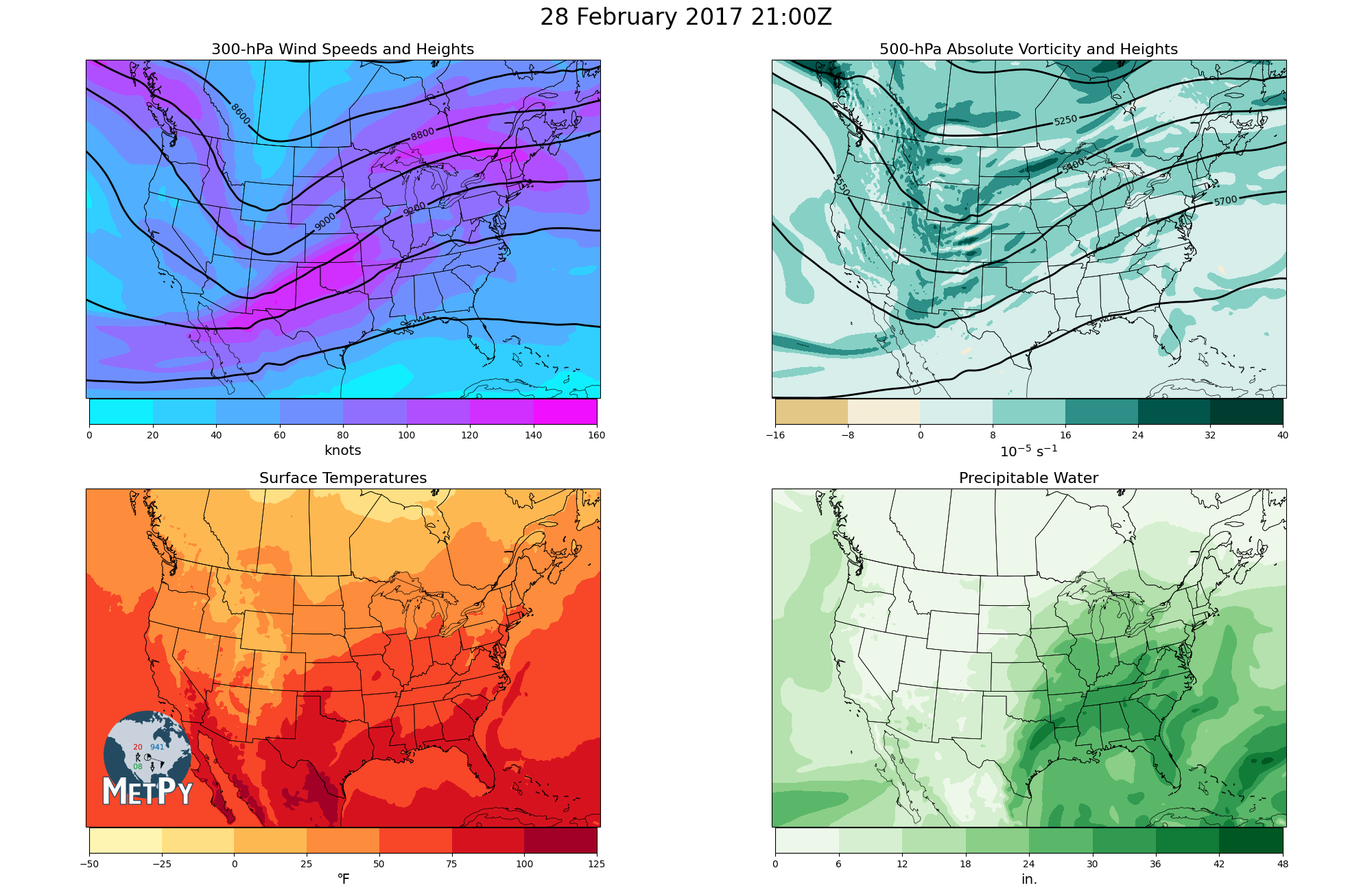
Four Panel Map#
By reading model output data from a netCDF file, we can create a four panel plot showing:
300 hPa heights and winds
500 hPa heights and absolute vorticity
Surface temperatures
Precipitable water
import cartopy.crs as ccrs
import cartopy.feature as cfeature
import matplotlib.pyplot as plt
import numpy as np
import scipy.ndimage as ndimage
import xarray as xr

from metpy.cbook import get_test_data
from metpy.plots import add_metpy_logo
crs = ccrs.LambertConformal(central_longitude=-100.0, central_latitude=45.0)
# Function used to create the map subplots
def plot_background(ax):
    ax.set_extent([235., 290., 20., 55.])
    ax.add_feature(cfeature.COASTLINE.with_scale('50m'), linewidth=0.5)
    ax.add_feature(cfeature.STATES, linewidth=0.5)
    ax.add_feature(cfeature.BORDERS, linewidth=0.5)
    return ax
# Open the example netCDF data
ds = xr.open_dataset(get_test_data('gfs_output.nc', False))
print(ds)
<xarray.Dataset> Size: 3MB
Dimensions:       (lat: 201, lon: 361, time: 1)
Coordinates:
  * lat           (lat) float32 804B 65.0 64.75 64.5 64.25 ... 15.5 15.25 15.0
  * lon           (lon) float32 1kB 220.0 220.2 220.5 ... 309.5 309.8 310.0
  * time          (time) datetime64[ns] 8B 2017-02-28T21:00:00
Data variables:
    temp          (time, lat, lon) float64 580kB ...
    precip_water  (time, lat, lon) float64 580kB ...
    heights_300   (time, lat, lon) float64 580kB ...
    heights_500   (time, lat, lon) float64 580kB ...
    vort_500      (time, lat, lon) float64 580kB ...
    winds_300     (time, lat, lon) float64 580kB ...
Attributes:
    title:     Test GFS Output Data
    subtitle:  For MetPy examples and tests
# Combine 1D latitude and longitudes into a 2D grid of locations
lon_2d, lat_2d = np.meshgrid(ds['lon'], ds['lat'])
# Pull out the data
vort_500 = ds['vort_500'][0]
surface_temp = ds['temp'][0]
precip_water = ds['precip_water'][0]
winds_300 = ds['winds_300'][0]
# Do unit conversions to what we wish to plot
vort_500 = vort_500 * 1e5
surface_temp = surface_temp.metpy.convert_units('degF')
precip_water = precip_water.metpy.convert_units('inches')
winds_300 = winds_300.metpy.convert_units('knots')
# Smooth the height data
heights_300 = ndimage.gaussian_filter(ds['heights_300'][0], sigma=1.5, order=0)
heights_500 = ndimage.gaussian_filter(ds['heights_500'][0], sigma=1.5, order=0)
# Create the figure and plot background on different axes
fig, axarr = plt.subplots(nrows=2, ncols=2, figsize=(20, 13), constrained_layout=True,
                          subplot_kw={'projection': crs})
add_metpy_logo(fig, 140, 120, size='large')
axlist = axarr.flatten()
for ax in axlist:
    plot_background(ax)

# Upper left plot - 300-hPa winds and geopotential heights
cf1 = axlist[0].contourf(lon_2d, lat_2d, winds_300, cmap='cool', transform=ccrs.PlateCarree())
c1 = axlist[0].contour(lon_2d, lat_2d, heights_300, colors='black', linewidths=2,
                       transform=ccrs.PlateCarree())
axlist[0].clabel(c1, fontsize=10, inline=1, inline_spacing=1, fmt='%i', rightside_up=True)
axlist[0].set_title('300-hPa Wind Speeds and Heights', fontsize=16)
cb1 = fig.colorbar(cf1, ax=axlist[0], orientation='horizontal', shrink=0.74, pad=0)
cb1.set_label('knots', size='x-large')

# Upper right plot - 500mb absolute vorticity and geopotential heights
cf2 = axlist[1].contourf(lon_2d, lat_2d, vort_500, cmap='BrBG', transform=ccrs.PlateCarree(),
                         zorder=0, norm=plt.Normalize(-32, 32))
c2 = axlist[1].contour(lon_2d, lat_2d, heights_500, colors='k', linewidths=2,
                       transform=ccrs.PlateCarree())
axlist[1].clabel(c2, fontsize=10, inline=1, inline_spacing=1, fmt='%i', rightside_up=True)
axlist[1].set_title('500-hPa Absolute Vorticity and Heights', fontsize=16)
cb2 = fig.colorbar(cf2, ax=axlist[1], orientation='horizontal', shrink=0.74, pad=0)
cb2.set_label(r'$10^{-5}$ s$^{-1}$', size='x-large')

# Lower left plot - surface temperatures
cf3 = axlist[2].contourf(lon_2d, lat_2d, surface_temp, cmap='YlOrRd',
                         transform=ccrs.PlateCarree(), zorder=0)
axlist[2].set_title('Surface Temperatures', fontsize=16)
cb3 = fig.colorbar(cf3, ax=axlist[2], orientation='horizontal', shrink=0.74, pad=0)
cb3.set_label('\N{DEGREE FAHRENHEIT}', size='x-large')

# Lower right plot - precipitable water entire atmosphere
cf4 = axlist[3].contourf(lon_2d, lat_2d, precip_water, cmap='Greens',
                         transform=ccrs.PlateCarree(), zorder=0)
axlist[3].set_title('Precipitable Water', fontsize=16)
cb4 = fig.colorbar(cf4, ax=axlist[3], orientation='horizontal', shrink=0.74, pad=0)
cb4.set_label('in.', size='x-large')

# Set height padding for plots
fig.set_constrained_layout_pads(w_pad=0., h_pad=0.1, hspace=0., wspace=0.)

# Set figure title
fig.suptitle(ds['time'][0].dt.strftime('%d %B %Y %H:%MZ').values, fontsize=24)

# Display the plot
plt.show()
Total running time of the script: (0 minutes 7.439 seconds)