
Note
Go to the end to download the full example code.
Cross Section Analysis#
The MetPy function metpy.interpolate.cross_section can obtain a cross-sectional slice through
gridded data.
import cartopy.crs as ccrs
import cartopy.feature as cfeature
import matplotlib.pyplot as plt
import numpy as np
import xarray as xr

import metpy.calc as mpcalc
from metpy.cbook import get_test_data
from metpy.interpolate import cross_section
Getting the data
This example uses [NARR reanalysis data]( https://www.ncei.noaa.gov/products/weather-climate-models/north-american-regional) for 18 UTC 04 April 1987 from NCEI.
We use MetPy’s CF parsing to get the data ready for use, and squeeze down the size-one time dimension.
data = xr.open_dataset(get_test_data('narr_example.nc', False))
data = data.metpy.parse_cf().squeeze()
print(data)
<xarray.Dataset> Size: 21MB
Dimensions:              (isobaric: 29, y: 118, x: 292)
Coordinates:
    time                 datetime64[ns] 8B 1987-04-04T18:00:00
  * isobaric             (isobaric) float64 232B 1e+03 975.0 ... 125.0 100.0
  * y                    (y) float64 944B -3.087e+06 -3.054e+06 ... 7.114e+05
  * x                    (x) float64 2kB -3.977e+06 -3.945e+06 ... 5.47e+06
    metpy_crs            object 8B Projection: lambert_conformal_conic
Data variables:
    Temperature          (isobaric, y, x) float32 4MB ...
    Lambert_Conformal    |S1 1B ...
    lat                  (y, x) float64 276kB ...
    lon                  (y, x) float64 276kB ...
    u_wind               (isobaric, y, x) float32 4MB ...
    v_wind               (isobaric, y, x) float32 4MB ...
    Geopotential_height  (isobaric, y, x) float32 4MB ...
    Specific_humidity    (isobaric, y, x) float32 4MB ...
Attributes: (12/14)
    Conventions:              CF-1.0
    Originating_center:       US National Weather Service - NCEP(WMC) (7)
    Originating_subcenter:    The North American Regional Reanalysis (NARR) P...
    Generating_Model:         North American Regional Reanalysis (NARR)
    Product_Type:             Forecast/Uninitialized Analysis/Image Product
    title:                    US National Weather Service - NCEP(WMC) North A...
    ...                       ...
    history:                  Direct read of GRIB-1 into NetCDF-Java 4 API
    CF:feature_type:          GRID
    file_format:              GRIB-1
    location:                 /nomads3_data/raid2/noaaport/merged/narr/198704...
    _CoordinateModelRunDate:  1987-04-04T18:00:00Z
    History:                  Translated to CF-1.0 Conventions by Netcdf-Java...
Define start and end points:
Get the cross section, and convert lat/lon to supplementary coordinates:
<xarray.Dataset> Size: 120kB
Dimensions:              (isobaric: 29, index: 100)
Coordinates:
    time                 datetime64[ns] 8B 1987-04-04T18:00:00
  * isobaric             (isobaric) float64 232B 1e+03 975.0 ... 125.0 100.0
    metpy_crs            object 8B Projection: lambert_conformal_conic
    x                    (index) float64 800B 1.818e+05 2.18e+05 ... 3.712e+06
    y                    (index) float64 800B -1.454e+06 ... -5.573e+05
  * index                (index) int64 800B 0 1 2 3 4 5 6 ... 94 95 96 97 98 99
    lat                  (index) float64 800B 37.0 37.05 37.11 ... 35.58 35.5
    lon                  (index) float64 800B -105.0 -104.6 ... -65.39 -65.0
Data variables:
    Temperature          (isobaric, index) float64 23kB 287.7 286.9 ... 211.4
    Lambert_Conformal    |S1 1B ...
    u_wind               (isobaric, index) float64 23kB -2.729 0.4776 ... 23.68
    v_wind               (isobaric, index) float64 23kB 8.473 5.723 ... -1.082
    Geopotential_height  (isobaric, index) float64 23kB 118.6 ... 1.636e+04
    Specific_humidity    (isobaric, index) float64 23kB 0.006367 ... 4.223e-06
Attributes: (12/14)
    Conventions:              CF-1.0
    Originating_center:       US National Weather Service - NCEP(WMC) (7)
    Originating_subcenter:    The North American Regional Reanalysis (NARR) P...
    Generating_Model:         North American Regional Reanalysis (NARR)
    Product_Type:             Forecast/Uninitialized Analysis/Image Product
    title:                    US National Weather Service - NCEP(WMC) North A...
    ...                       ...
    history:                  Direct read of GRIB-1 into NetCDF-Java 4 API
    CF:feature_type:          GRID
    file_format:              GRIB-1
    location:                 /nomads3_data/raid2/noaaport/merged/narr/198704...
    _CoordinateModelRunDate:  1987-04-04T18:00:00Z
    History:                  Translated to CF-1.0 Conventions by Netcdf-Java...
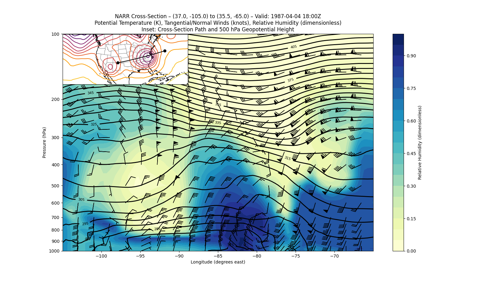
For this example, we will be plotting potential temperature, relative humidity, and tangential/normal winds. And so, we need to calculate those, and add them to the dataset:
cross['Potential_temperature'] = mpcalc.potential_temperature(
    cross['isobaric'],
    cross['Temperature']
)
cross['Relative_humidity'] = mpcalc.relative_humidity_from_specific_humidity(
    cross['isobaric'],
    cross['Temperature'],
    cross['Specific_humidity']
)
cross['u_wind'] = cross['u_wind'].metpy.convert_units('knots')
cross['v_wind'] = cross['v_wind'].metpy.convert_units('knots')
cross['t_wind'], cross['n_wind'] = mpcalc.cross_section_components(
    cross['u_wind'],
    cross['v_wind']
)

print(cross)
<xarray.Dataset> Size: 213kB
Dimensions:                (isobaric: 29, index: 100)
Coordinates:
    time                   datetime64[ns] 8B 1987-04-04T18:00:00
  * isobaric               (isobaric) float64 232B 1e+03 975.0 ... 125.0 100.0
    metpy_crs              object 8B Projection: lambert_conformal_conic
    x                      (index) float64 800B 1.818e+05 2.18e+05 ... 3.712e+06
    y                      (index) float64 800B -1.454e+06 ... -5.573e+05
  * index                  (index) int64 800B 0 1 2 3 4 5 ... 94 95 96 97 98 99
    lat                    (index) float64 800B 37.0 37.05 37.11 ... 35.58 35.5
    lon                    (index) float64 800B -105.0 -104.6 ... -65.39 -65.0
Data variables:
    Temperature            (isobaric, index) float64 23kB 287.7 286.9 ... 211.4
    Lambert_Conformal      |S1 1B ...
    u_wind                 (isobaric, index) float64 23kB <Quantity([[ -5.304...
    v_wind                 (isobaric, index) float64 23kB <Quantity([[16.4704...
    Geopotential_height    (isobaric, index) float64 23kB 118.6 ... 1.636e+04
    Specific_humidity      (isobaric, index) float64 23kB 0.006367 ... 4.223e-06
    Potential_temperature  (isobaric, index) float64 23kB <Quantity([[287.717...
    Relative_humidity      (isobaric, index) float64 23kB <Quantity([[0.61567...
    t_wind                 (isobaric, index) float64 23kB <Quantity([[-2.0266...
    n_wind                 (isobaric, index) float64 23kB <Quantity([[ 17.184...
Attributes: (12/14)
    Conventions:              CF-1.0
    Originating_center:       US National Weather Service - NCEP(WMC) (7)
    Originating_subcenter:    The North American Regional Reanalysis (NARR) P...
    Generating_Model:         North American Regional Reanalysis (NARR)
    Product_Type:             Forecast/Uninitialized Analysis/Image Product
    title:                    US National Weather Service - NCEP(WMC) North A...
    ...                       ...
    history:                  Direct read of GRIB-1 into NetCDF-Java 4 API
    CF:feature_type:          GRID
    file_format:              GRIB-1
    location:                 /nomads3_data/raid2/noaaport/merged/narr/198704...
    _CoordinateModelRunDate:  1987-04-04T18:00:00Z
    History:                  Translated to CF-1.0 Conventions by Netcdf-Java...
Now, we can make the plot.
# Define the figure object and primary axes
fig = plt.figure(1, figsize=(16., 9.))
ax = plt.axes()

# Plot RH using contourf
rh_contour = ax.contourf(cross['lon'], cross['isobaric'], cross['Relative_humidity'],
                         levels=np.arange(0, 1.05, .05), cmap='YlGnBu')
rh_colorbar = fig.colorbar(rh_contour)

# Plot potential temperature using contour, with some custom labeling
theta_contour = ax.contour(cross['lon'], cross['isobaric'], cross['Potential_temperature'],
                           levels=np.arange(250, 450, 5), colors='k', linewidths=2)
theta_contour.clabel(theta_contour.levels[1::2], fontsize=8, colors='k', inline=1,
                     inline_spacing=8, fmt='%i', rightside_up=True, use_clabeltext=True)

# Plot winds using the axes interface directly, with some custom indexing to make the barbs
# less crowded
wind_slc_vert = list(range(0, 19, 2)) + list(range(19, 29))
wind_slc_horz = slice(5, 100, 5)
ax.barbs(cross['lon'][wind_slc_horz], cross['isobaric'][wind_slc_vert],
         cross['t_wind'][wind_slc_vert, wind_slc_horz],
         cross['n_wind'][wind_slc_vert, wind_slc_horz], color='k')

# Adjust the y-axis to be logarithmic
ax.set_yscale('symlog')
ax.set_ylim(cross['isobaric'].max(), cross['isobaric'].min())
ax.set_yticks(np.arange(1000, 50, -100))

# Define the CRS and inset axes
data_crs = data['Geopotential_height'].metpy.cartopy_crs
ax_inset = fig.add_axes([0.125, 0.665, 0.25, 0.25], projection=data_crs)

# Plot geopotential height at 500 hPa using xarray's contour wrapper
ax_inset.contour(data['x'], data['y'], data['Geopotential_height'].sel(isobaric=500.),
                 levels=np.arange(5100, 6000, 60), cmap='inferno')

# Plot the path of the cross section
endpoints = data_crs.transform_points(ccrs.Geodetic(),
                                      *np.vstack([start, end]).transpose()[::-1])
ax_inset.scatter(endpoints[:, 0], endpoints[:, 1], c='k', zorder=2)
ax_inset.plot(cross['x'], cross['y'], c='k', zorder=2)

# Add geographic features
ax_inset.coastlines()
ax_inset.add_feature(cfeature.STATES.with_scale('50m'), edgecolor='k', alpha=0.2, zorder=0)

# Set the titles and axes labels
ax_inset.set_title('')
ax.set_title(f'NARR Cross-Section \u2013 {start} to {end} \u2013 '
             f'Valid: {cross["time"].dt.strftime("%Y-%m-%d %H:%MZ").item()}\n'
             'Potential Temperature (K), Tangential/Normal Winds (knots), Relative Humidity '
             '(dimensionless)\nInset: Cross-Section Path and 500 hPa Geopotential Height')
ax.set_ylabel('Pressure (hPa)')
ax.set_xlabel('Longitude (degrees east)')
rh_colorbar.set_label('Relative Humidity (dimensionless)')

plt.show()
Note: The x-axis can display any variable that is the same length as the
plotted variables, including latitude. Additionally, arguments can be provided
to ax.set_xticklabels to label lat/lon pairs, similar to the default NCL output.
Total running time of the script: (0 minutes 4.376 seconds)