
Note
Go to the end to download the full example code.
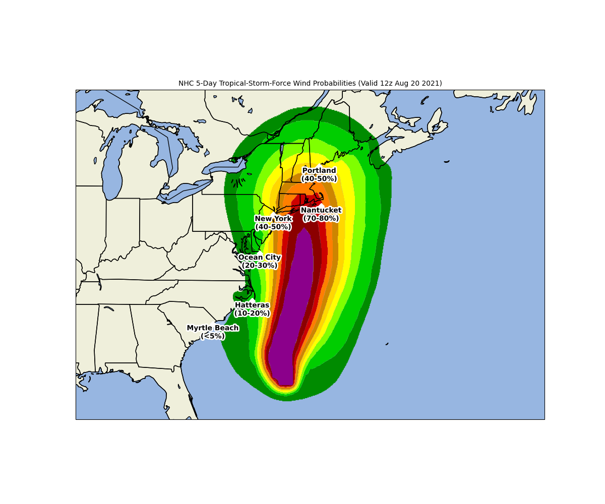
NOAA NHC Wind Speed Probabilities#
Demonstrate the use of geoJSON and shapefile data with PlotGeometry in MetPy’s simplified plotting interface. This example walks through plotting cities, along with 5-day tropical-storm-force wind speed probabilities from NOAA National Hurricane Center.
The wind probabilities shapefile was retrieved from the National Hurricane Center’s GIS page. The cities shapefile was retrieved from Stanford Libraries.
import geopandas

from metpy.cbook import get_test_data
from metpy.plots import MapPanel, PanelContainer, PlotGeometry
Read in the shapefile file containing the wind probabilities.
wind_data = geopandas.read_file(get_test_data('nhc_wind_prob_2021082012.zip'))
/opt/hostedtoolcache/Python/3.13.7/x64/lib/python3.13/site-packages/pyogrio/geopandas.py:275: UserWarning: More than one layer found in 'pyogrio_d6c04cd67d1140bd827b47712d9ca94a.zip': '2021082012_wsp34knt120hr_5km' (default), '2021082012_wsp50knt120hr_5km', '2021082012_wsp64knt120hr_5km'. Specify layer parameter to avoid this warning.
  result = read_func(
Add the color scheme to the GeoDataFrame. This is the same color scheme used by the National Hurricane Center for their wind speed probability plots.
wind_data['fill'] = ['none', '#008B00', '#00CD00', '#7FFF00', '#FFFF00', '#FFD700',
                     '#CD8500', '#FF7F00', '#CD0000', '#8B0000', '#8B008B']
wind_data
Read in the shapefile file containing the cities.
cities = geopandas.read_file(get_test_data('us_cities.zip'))
There are thousands of cities in the United States. We choose a few cities here that we want to display on our plot.
cities = cities.loc[
    ((cities['NAME'] == 'Myrtle Beach') & (cities['STATE'] == 'SC'))
    | ((cities['NAME'] == 'Hatteras') & (cities['STATE'] == 'NC'))
    | ((cities['NAME'] == 'Ocean City') & (cities['STATE'] == 'MD'))
    | ((cities['NAME'] == 'New York') & (cities['STATE'] == 'NY'))
    | ((cities['NAME'] == 'Nantucket') & (cities['STATE'] == 'MA'))
    | ((cities['NAME'] == 'Portland') & (cities['STATE'] == 'ME'))
]
cities
Make sure that both GeoDataFrames have the same coordinate reference system (CRS).
cities = cities.to_crs(wind_data.crs)
We want to find out what the probability of tropical-storm-force winds is for each of the cities we selected above. Geopandas provides a spatial join method, which merges the two GeoDataFrames and can tell us which wind speed probability polygon each of our city points lies within. That information is stored in the ‘PERCENTAGE’ column below.
cities = geopandas.sjoin(cities, wind_data, how='left', predicate='within')
cities
Plot the wind speed probability polygons from the ‘geometry’ column. Use the ‘fill’ column we created above as the fill colors for the polygons, and set the stroke color to ‘none’ for all of the polygons.
wind_geo = PlotGeometry()
wind_geo.geometry = wind_data['geometry']
wind_geo.fill = wind_data['fill']
wind_geo.stroke = 'none'
Plot the cities from the ‘geometry’ column, marked with diamonds (‘D’). Label each point with the name of the city, and it’s probability of tropical-storm-force winds on the line below. Points are set to plot in white and the font color is set to black.
city_geo = PlotGeometry()
city_geo.geometry = cities['geometry']
city_geo.marker = 'D'
city_geo.labels = cities['NAME'] + '\n(' + cities['PERCENTAGE'] + ')'
city_geo.fill = 'white'
city_geo.label_facecolor = 'black'
Add the geometry plots to a panel and container. Finally, we are left with a complete plot of wind speed probabilities, along with some select cities and their specific probabilities.
panel = MapPanel()
panel.title = 'NHC 5-Day Tropical-Storm-Force Wind Probabilities (Valid 12z Aug 20 2021)'
panel.plots = [wind_geo, city_geo]
panel.area = [-90, -52, 27, 48]
panel.projection = 'mer'
panel.layers = ['lakes', 'land', 'ocean', 'states', 'coastline', 'borders']

pc = PanelContainer()
pc.size = (12, 10)
pc.panels = [panel]
pc.show()
Total running time of the script: (0 minutes 5.872 seconds)