
Note
Go to the end to download the full example code.
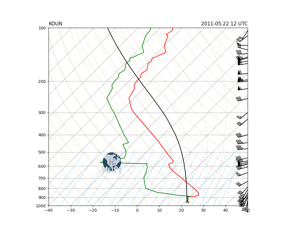
Sounding as Dataset Example#
Use MetPy to make a Skew-T LogP plot from an xarray Dataset after computing LCL parcel profile.
This example makes a skewT diagram with specified special lines while storing the sounding data as an xarray dataset.
import matplotlib.pyplot as plt
import numpy as np
import pandas as pd

import metpy.calc as mpcalc
from metpy.cbook import get_test_data
from metpy.plots import add_metpy_logo, SkewT
from metpy.units import units
Upper air data can be obtained using the siphon package, but for this example we will use some of MetPy’s sample data.
col_names = ['pressure', 'height', 'temperature', 'dewpoint', 'direction', 'speed']

df = pd.read_fwf(get_test_data('20110522_OUN_12Z.txt', as_file_obj=False),
                 skiprows=7, usecols=[0, 1, 2, 3, 6, 7], names=col_names)

# Drop any rows with all NaN values for T, Td, winds
df = df.dropna(subset=('temperature', 'dewpoint', 'direction', 'speed'),
               how='all').reset_index(drop=True)
We will pull the data out of the example dataset into individual variables and assign units.
p = df['pressure'].values * units.hPa
T = df['temperature'].values * units.degC
Td = df['dewpoint'].values * units.degC
wind_speed = df['speed'].values * units.knots
wind_dir = df['direction'].values * units.degrees
u, v = mpcalc.wind_components(wind_speed, wind_dir)

ds = mpcalc.parcel_profile_with_lcl_as_dataset(p, T, Td)
print(list(ds.variables))
['ambient_temperature', 'ambient_dew_point', 'parcel_temperature', 'isobaric']
fig = plt.figure(figsize=(10, 8))
skew = SkewT(fig, rotation=45)

# Plot the data using the data from the xarray Dataset including the parcel temperature with
# the LCL level included
skew.plot(ds.isobaric, ds.ambient_temperature, 'r')
skew.plot(ds.isobaric, ds.ambient_dew_point, 'g')
skew.plot(ds.isobaric, ds.parcel_temperature.metpy.convert_units('degC'), 'black')

# Plot the wind barbs from the original data
skew.plot_barbs(p[::2], u[::2], v[::2])

# Add the relevant special lines
pressure = np.arange(1000, 499, -50) * units('hPa')
mixing_ratio = np.array([0.1, 0.2, 0.4, 0.6, 1, 1.5, 2, 3, 4,
                        6, 8, 10, 13, 16, 20, 25, 30, 36, 42]).reshape(-1, 1) * units('g/kg')

skew.plot_dry_adiabats(t0=np.arange(233, 533, 10) * units.K, alpha=0.25,
                       colors='orangered', linewidths=1)
skew.plot_moist_adiabats(t0=np.arange(233, 400, 5) * units.K, alpha=0.25,
                         colors='tab:green', linewidths=1)
skew.plot_mixing_lines(pressure=pressure, mixing_ratio=mixing_ratio, linestyles='dotted',
                       colors='dodgerblue', linewidths=1)
skew.ax.set_ylim(1000, 100)

# Add the MetPy logo!
add_metpy_logo(fig, 350, 200)

# Add some titles
plt.title('KOUN', loc='left')
plt.title('2011-05-22 12 UTC', loc='right')

plt.show()
/opt/hostedtoolcache/Python/3.13.7/x64/lib/python3.13/site-packages/scipy/integrate/_ivp/base.py:23: UserWarning: Saturation mixing ratio is undefined for some requested pressure/temperature combinations. Total pressure must be greater than the water vapor saturation pressure for liquid water to be in equilibrium.
  return np.asarray(fun(t, y), dtype=dtype)
/opt/hostedtoolcache/Python/3.13.7/x64/lib/python3.13/site-packages/metpy/calc/thermo.py:1633: RuntimeWarning: invalid value encountered in power
  * (mpconsts.nounit.T0 / temperature) ** heat_power
Total running time of the script: (0 minutes 0.186 seconds)