
Note
Go to the end to download the full example code.
Simple Plotting of Fronts#
This uses MetPy’s path effects for matplotlib that can be used to represent a line as a traditional front. This example relies on already having location information for the boundaries you would like to plot.
Define some synthetic points to represent the low pressure system and its frontal boundaries.
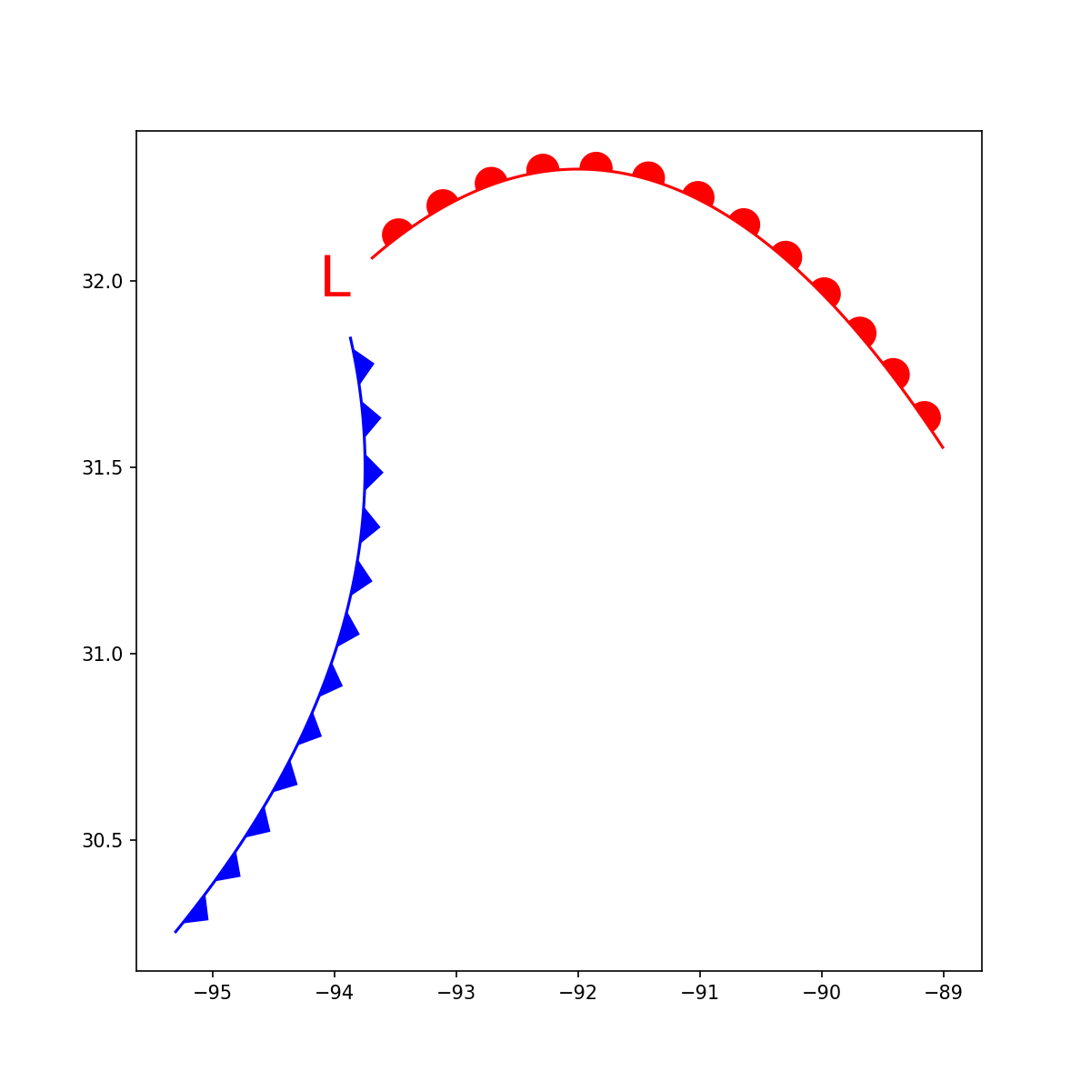
Draw the low as an “L” using matplotlib’s text() method, then plot the fronts as standard lines, but add our path effects.
fig, ax = plt.subplots(figsize=(8, 8), dpi=150)
ax.text(low_lon, low_lat, 'L', color='red', size=30,
        horizontalalignment='center', verticalalignment='center')
ax.plot(cold_lon, cold_lat, 'blue', path_effects=[ColdFront(size=8, spacing=1.5)])
ax.plot(warm_lon, warm_lat, 'red', path_effects=[WarmFront(size=8, spacing=1.5)])
plt.show()
Total running time of the script: (0 minutes 0.098 seconds)