Note
Go to the end to download the full example code.
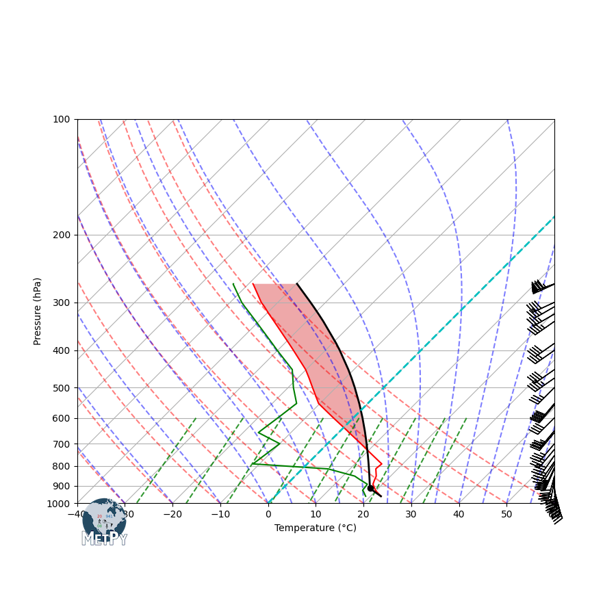
Advanced Sounding#
Plot a sounding using MetPy with more advanced features.
Beyond just plotting data, this uses calculations from metpy.calc to find the lifted
condensation level (LCL) and the profile of a surface-based parcel. The area between the
ambient profile and the parcel profile is colored as well.
import matplotlib.pyplot as plt
import pandas as pd

import metpy.calc as mpcalc
from metpy.cbook import get_test_data
from metpy.plots import add_metpy_logo, SkewT
from metpy.units import units
Upper air data can be obtained using the siphon package, but for this example we will use some of MetPy’s sample data.
col_names = ['pressure', 'height', 'temperature', 'dewpoint', 'direction', 'speed']

df = pd.read_fwf(get_test_data('may4_sounding.txt', as_file_obj=False),
                 skiprows=5, usecols=[0, 1, 2, 3, 6, 7], names=col_names)

# Drop any rows with all NaN values for T, Td, winds
df = df.dropna(subset=('temperature', 'dewpoint', 'direction', 'speed'), how='all'
               ).reset_index(drop=True)
We will pull the data out of the example dataset into individual variables and assign units.
p = df['pressure'].values * units.hPa
T = df['temperature'].values * units.degC
Td = df['dewpoint'].values * units.degC
wind_speed = df['speed'].values * units.knots
wind_dir = df['direction'].values * units.degrees
u, v = mpcalc.wind_components(wind_speed, wind_dir)
Create a new figure. The dimensions here give a good aspect ratio.
fig = plt.figure(figsize=(9, 9))
add_metpy_logo(fig, 115, 100)
skew = SkewT(fig, rotation=45)

# Plot the data using normal plotting functions, in this case using
# log scaling in Y, as dictated by the typical meteorological plot.
skew.plot(p, T, 'r')
skew.plot(p, Td, 'g')
skew.plot_barbs(p, u, v)
skew.ax.set_ylim(1000, 100)
skew.ax.set_xlim(-40, 60)

# Set some better labels than the default
skew.ax.set_xlabel(f'Temperature ({T.units:~P})')
skew.ax.set_ylabel(f'Pressure ({p.units:~P})')

# Calculate LCL height and plot as black dot. Because `p`'s first value is
# ~1000 mb and its last value is ~250 mb, the `0` index is selected for
# `p`, `T`, and `Td` to lift the parcel from the surface. If `p` was inverted,
# i.e. start from low value, 250 mb, to a high value, 1000 mb, the `-1` index
# should be selected.
lcl_pressure, lcl_temperature = mpcalc.lcl(p[0], T[0], Td[0])
skew.plot(lcl_pressure, lcl_temperature, 'ko', markerfacecolor='black')

# Calculate full parcel profile and add to plot as black line
prof = mpcalc.parcel_profile(p, T[0], Td[0]).to('degC')
skew.plot(p, prof, 'k', linewidth=2)

# Shade areas of CAPE and CIN
skew.shade_cin(p, T, prof, Td)
skew.shade_cape(p, T, prof)

# An example of a slanted line at constant T -- in this case the 0
# isotherm
skew.ax.axvline(0, color='c', linestyle='--', linewidth=2)

# Add the relevant special lines
skew.plot_dry_adiabats()
skew.plot_moist_adiabats()
skew.plot_mixing_lines()

# Show the plot
plt.show()
Total running time of the script: (0 minutes 0.180 seconds)