METAR Station Plot with MetPy
Notebook Python-AWIPS Tutorial Notebook
Objectives
Use python-awips to connect to an edex server
Define and filter data request for METAR surface obs
Extract necessary data and reformat it for plotting
Stylize and plot METAR station data using Cartopy, Matplotlib, and MetPy
Table of Contents
1 Imports
The imports below are used throughout the notebook. Note the first two imports are coming directly from python-awips and allow us to connect to an EDEX server, and define a timrange used for filtering the data. The subsequent imports are for data manipulation and visualization.
from awips.dataaccess import DataAccessLayer
from dynamicserialize.dstypes.com.raytheon.uf.common.time import TimeRange
from datetime import datetime, timedelta, UTC
import numpy as np
import cartopy.crs as ccrs
import cartopy.feature as cfeature
import matplotlib.pyplot as plt
from metpy.calc import wind_components
from metpy.plots import StationPlot, StationPlotLayout, sky_cover
from metpy.units import units
2 Function: get_cloud_cover()
Returns the cloud coverage values as integer codes (0 through 8).
def get_cloud_cover(code):
    if 'OVC' in code:
        return 8
    elif 'BKN' in code:
        return 6
    elif 'SCT' in code:
        return 4
    elif 'FEW' in code:
        return 2
    else:
        return 0
3 Initial Setup
3.1 Initial EDEX Connection
First we establish a connection to Unidata’s public EDEX server. With that connection made, we can create a new data request object and set the data type to obs.
Then, because we’re going to uses MetPy’s StationPlot and StationPlotLayout we need to define several parameters, and then set them on the data request object.
# EDEX Request
edexServer = "edex-cloud.unidata.ucar.edu"
DataAccessLayer.changeEDEXHost(edexServer)
request = DataAccessLayer.newDataRequest("obs")

# define desired parameters
single_value_params = ["stationName", "longitude", "latitude",
                       "temperature", "dewpoint", "windDir",
                       "windSpeed"]
multi_value_params = ["skyCover"]

params = single_value_params + multi_value_params

# set all parameters on the request
request.setParameters(*(params))
3.2 Setting Connection Location Names
We are also going to define specific station IDs so that our plot is not too cluttered.
# Define a list of station IDs to plot
selected = ['KPDX', 'KOKC', 'KICT', 'KGLD', 'KMEM', 'KBOS', 'KMIA', 'KMOB', 'KABQ', 'KPHX', 'KTTF',
            'KORD', 'KBIL', 'KBIS', 'KCPR', 'KLAX', 'KATL', 'KMSP', 'KSLC', 'KDFW', 'KNYC', 'KPHL',
            'KPIT', 'KIND', 'KOLY', 'KSYR', 'KLEX', 'KCHS', 'KTLH', 'KHOU', 'KGJT', 'KLBB', 'KLSV',
            'KGRB', 'KCLT', 'KLNK', 'KDSM', 'KBOI', 'KFSD', 'KRAP', 'KRIC', 'KJAN', 'KHSV', 'KCRW',
            'KSAT', 'KBUY', 'K0CO', 'KZPC', 'KVIH', 'KBDG', 'KMLF', 'KELY', 'KWMC', 'KOTH', 'KCAR',
            'KLMT', 'KRDM', 'KPDT', 'KSEA', 'KUIL', 'KEPH', 'KPUW', 'KCOE', 'KMLP', 'KPIH', 'KIDA',
            'KMSO', 'KACV', 'KHLN', 'KBIL', 'KOLF', 'KRUT', 'KPSM', 'KJAX', 'KTPA', 'KSHV', 'KMSY',
            'KELP', 'KRNO', 'KFAT', 'KSFO', 'KNYL', 'KBRO', 'KMRF', 'KDRT', 'KFAR', 'KBDE', 'KDLH',
            'KHOT', 'KLBF', 'KFLG', 'KCLE', 'KUNV']

# set the location names to the desired station IDs
request.setLocationNames(*(selected))
4 Filter by Time
Here we decide how much data we want to pull from EDEX. By default we’ll
request 1 hour, but that value can easily be modified by adjusting the
``timedelta(hours = 1)` <https://docs.python.org/3/library/datetime.html#timedelta-objects>`__
in line 2. The more data we request, the longer this section will
take to run.
# Time range
lastHourDateTime = datetime.now(UTC) - timedelta(hours = 1)
start = lastHourDateTime.strftime('%Y-%m-%d %H')
beginRange = datetime.strptime( start + ":00:00", "%Y-%m-%d %H:%M:%S")
endRange = datetime.strptime( start + ":59:59", "%Y-%m-%d %H:%M:%S")
timerange = TimeRange(beginRange, endRange)
5 Use the Data!
5.1 Get the Data!
Now that we have our request and TimeRange timerange objects
ready, we’re ready to get the data array from EDEX.
# Get response
response = DataAccessLayer.getGeometryData(request,timerange)
5.2 Extract all Parameters
In this section we start gathering all the information we’ll need to
properly display our data. First we create an empty dictionary and array
to keep track of all data and unique station IDs. We also create a
boolean to help us only grab the first entry for skyCover related to
a station id.
Note: The way the data responses are returned, we recieve many
skyCoverentries for each station ID, but we only want to keep track of the most recent one (first one returned).
After defining these variables, we are ready to start looping through
our response data. If the response is an entry of skyCover, and this
is a new station id, then set the skyCover value in the obs dictionary.
If this is not a skyCover entry, then explicitly set the timeObs
variable (because we have to manipulate it slightly), and dynamically
set all the remaining parameters.
# define a dictionary and array that will be populated from our for loop below
obs = dict({params: [] for params in params})
station_names = []
time_title = ""
i = 0

# cycle through all the data in the response, in reverse order to get the most recent data first
for ob in reversed(response):
    avail_params = ob.getParameters()
    #print(avail_params)
    # if it has cloud information, we want the last of the 6 entries (most recent)
    if "skyCover" in avail_params:
        if i == 5:
            # store the associated cloud cover int for the skyCover string
            obs['skyCover'].append(get_cloud_cover(ob.getString("skyCover")))
        i = i + 1
    elif "stationName" in avail_params:
        # If we already have a record for this stationName, skip
        if ob.getString('stationName') not in station_names:
            station_names.append(ob.getString('stationName'))
            i = 0
            if time_title == "":
                time_title = str(ob.getDataTime())
            for param in single_value_params:
                if param in avail_params:
                    try:
                        obs[param].append(ob.getNumber(param))
                    except TypeError:
                        obs[param].append(ob.getString(param))
                else:
                    obs[param].append(None)
5.3 Populate the Data Dictionary
Next grab the variables out of the obs dictionary we just populated, attach correct units, (calculate their components, in the instance of wind) and put them into a new dictionary that we will hand the plotting function later.
data = dict()
data['stid'] = np.array(obs['stationName'])
data['latitude']  = np.array(obs['latitude'])
data['longitude'] = np.array(obs['longitude'])
data['air_temperature'] = np.array(obs['temperature'], dtype=float)* units.degC
data['dew_point_temperature'] = np.array(obs['dewpoint'], dtype=float)* units.degC

direction = np.array(obs['windDir'])
direction[direction == -9999.0] = 'nan'

u, v = wind_components(np.array(obs['windSpeed']) * units('knots'),
                           direction * units.degree)
data['eastward_wind'], data['northward_wind'] = u, v
data['cloud_coverage'] = np.array(obs['skyCover'])
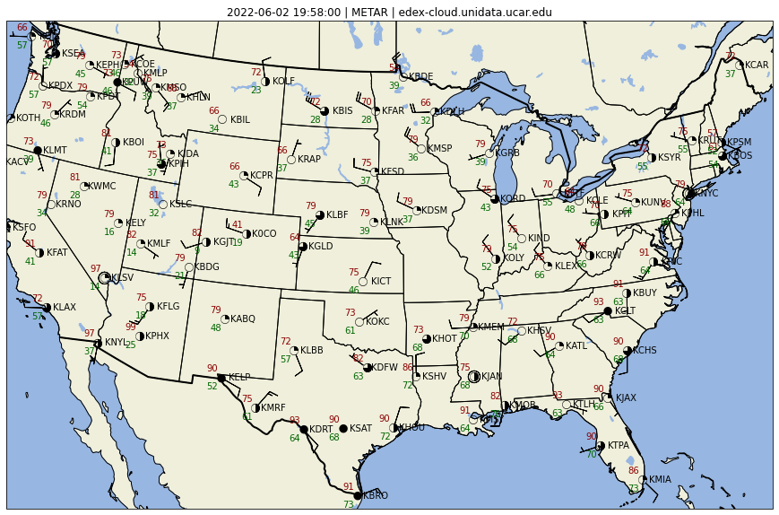
6 Plot the Data!
Now we have all the data we need to create our plot! First we’ll assign a projection and create our figure and axes.
Next, we use Cartopy to add common features (land, ocean, lakes, borders, etc) to help give us a more contextual map of the United States to plot the METAR stations on. We create and add a title for our figure as well.
Additionally, we use MetPy’s StationPlotLayout to instantiate a custom layout and define all the attributes we want displayed. We need to then set the data dictionary (containing all of our data values) on the custom layout so it knows what to draw.
Finally, we display the plot!
proj = ccrs.LambertConformal(central_longitude=-95, central_latitude=35,
                             standard_parallels=[35])
# Create the figure
fig = plt.figure(figsize=(20, 10))
ax = fig.add_subplot(1, 1, 1, projection=proj)

# Add various map elements
ax.add_feature(cfeature.LAND)
ax.add_feature(cfeature.OCEAN)
ax.add_feature(cfeature.LAKES)
ax.add_feature(cfeature.COASTLINE)
ax.add_feature(cfeature.STATES)
ax.add_feature(cfeature.BORDERS, linewidth=2)

# Set plot bounds
ax.set_extent((-118, -73, 23, 50))
ax.set_title(time_title + " | METAR | " + edexServer)

# Winds, temps, dewpoint, station id
custom_layout = StationPlotLayout()
custom_layout.add_barb('eastward_wind', 'northward_wind', units='knots')
custom_layout.add_value('NW', 'air_temperature', fmt='.0f', units='degF', color='darkred')
custom_layout.add_value('SW', 'dew_point_temperature', fmt='.0f', units='degF', color='darkgreen')
custom_layout.add_symbol('C', 'cloud_coverage', sky_cover)

stationplot = StationPlot(ax, data['longitude'], data['latitude'], clip_on=True,
                          transform=ccrs.PlateCarree(), fontsize=10)
stationplot.plot_text((2, 0), data['stid'])
custom_layout.plot(stationplot, data)

plt.show()
7 See Also
7.2 Additional Documentation
python-awips:
datetime:
numpy:
cartopy:
matplotlib:
metpy: