Click here to launch an
interactive online version of this notebook:
Rapid moistening of column water vapor: what’s going on there?
Drilling down into the science of:
Mapes, B. E., Chung, E. S., Hannah, W. M., Masunaga, H., Wimmers, A. J., & Velden, C. S. (2018). The meandering margin of the meteorological moist tropics. Geophysical Research Letters, 45. https://doi.org/10.1002/2017GL07644. Free ReadCube viewing at http://rdcu.be/GpqN.
Steps in the analysis
Importing CWV and AT data
Joint distributions
Build clickable maps in Holoviews
Clickable maps of high AT scenes
[1]:
import numpy as np
import matplotlib.pyplot as plt
import xarray as xr
from datetime import datetime
from datetime import timedelta
from IPython.display import HTML,display
[2]:
%matplotlib inline
Open the daily (v4) MIMIC-AT dataset
download from here for speed, or use the OpenDAP link in the code cell below
MIMIC-AT Repository, or here as a single datafile
[3]:
###REMOTE DATASET: 2 years
da = xr.open_dataset('https://weather.rsmas.miami.edu/repository/opendap/synth:0ce7321c-8278-47ef-bb56-7db18c21ea7d:L01JTUlDX0FUX2RhaWx5LjIwMTUtMjAxNl8yZGVnLm5jbWw=/entry.das')
###REMOTE DATASET: 1 month
#da=xr.open_dataset('http://weather.rsmas.miami.edu/repository/opendap/synth:0ce7321c-8278-47ef-bb56-7db18c21ea7d:L01JTUlDLndpdGhfQVQudjQuMjAxNzAzLm5j/entry.das')
###Open local dataset if you downloaded it first
#da=xr.open_dataset('MIMIC.with_AT.v4.2015-2016.2deg_lattrunc.nc')
da
- execution-count
3
<xarray.Dataset> Dimensions: (lat: 90, lon: 180, time: 730) Coordinates: * lon (lon) float64 0.0 2.0 4.0 6.0 8.0 10.0 12.0 14.0 16.0 18.0 ... * lat (lat) float64 -89.0 -87.0 -85.0 -83.0 -81.0 -79.0 -77.0 -75.0 ... * time (time) datetime64[ns] 2015-01-01T12:00:00 2015-01-02T12:00:00 ... Data variables: TPW_TEND (time, lat, lon) float64 ... mosaicTPW (time, lat, lon) float64 ... Attributes: CDI: Climate Data Interface version 1.6.4 (http://code.zmaw.de/p... Conventions: CF-1.4 history: Thu Apr 12 20:02:33 2018: cdo remapcon,r180x90 MIMIC.with_A... CDO: Climate Data Operators version 1.6.4 (http://code.zmaw.de/p...
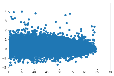
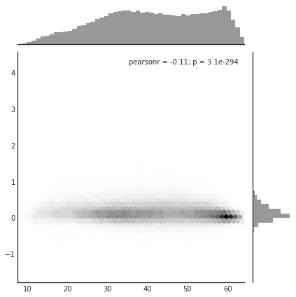
## General character of the data ### Joint histogram of TPW and its Lagrangian tendency
[4]:
subset = da.sel(time=slice(datetime(2015,1,1),datetime(2015,1,30)))\
.sel(lat =slice(-30,30))
x = subset.mosaicTPW.data
y = subset.TPW_TEND.data
plt.scatter(x,y); plt.xlim(30,70)
[4]:
(30, 70)
[5]:
# To get marginals (see skew and bimodality), use Seaborn
import pandas as pd
import seaborn as sns
# sns.set(color_codes=True)
df = pd.DataFrame({'x': [x], 'y': [y] })
with sns.axes_style("white"):
sns.jointplot(x=x, y=y, kind="hex", color="k");
Utilities: make clickable map
[6]:
import holoviews as hv
from bokeh.models import OpenURL, TapTool, HoverTool
hv.notebook_extension('bokeh')


make custom function for drawing coastlines
[7]:
def coastlines(resolution='110m',lon_360=False):
""" A custom method to plot in cylyndrical equi projection, most useful for
native projections, geoviews currently supports only Web Mercator in
bokeh mode.
Other resolutions can be 50m
lon_360 flag specifies if longitudes are from -180 to 180 (default) or 0 to 360
TODO: if hv.Polygons is used instead of overlay it is way faster but
something is wrong there.
"""
try:
import cartopy.io.shapereader as shapereader
from cartopy.io.shapereader import natural_earth
import shapefile
filename = natural_earth(resolution=resolution,category='physical',name='coastline')
sf = shapefile.Reader(filename)
fields = [x[0] for x in sf.fields][1:]
records = sf.records()
shps = [s.points for s in sf.shapes()]
pls=[]
for shp in shps:
lons=[lo for lo,_ in shp]
lats=[la for _,la in shp]
if lon_360:
lats_patch1=[lat for lon,lat in zip(lons,lats) if lon<0]
lons_patch1=[lon+360.0 for lon in lons if lon<0]
if any(lons_patch1):
pls.append(hv.Path((lons_patch1,lats_patch1))(style={'color':'Black'}))
lats_patch2=[lat if lon>=0 else None for lon,lat in zip(lons,lats)]
lons_patch2=[lon if lon>=0 else None for lon in lons]
if any(lons_patch2):
pls.append(hv.Path((lons_patch2,lats_patch2))(style={'color':'Black'}))
else:
pls.append(hv.Path((lons,lats))(style={'color':'Black'}))
return hv.Overlay(pls)
except Exception as err:
print('Overlaying Coastlines not available from holoviews because: {0}'.format(err))
[8]:
coastline=coastlines(lon_360=True) #this may download shape files on first invocation
#if data longitudes are -180 to 180 then lon_360=False
Create some tools to attach to the plots: hover tool for values
[9]:
hover = HoverTool(
tooltips=[
("Time", "@eventtimestr"),
("(Lat,Lon)", "(Lon=@eventlonstr{0[.]00}, Lat=@eventlatstr{0[.]00})"),
("TPW_TEND","@TPW_TEND"),
("TPW","@mosaicTPW")
]
)
#gives info on hovering on a location in the plot
Create some tools to attach to the plots: tap tool calls the NASA URL!
[10]:
tptool=TapTool()
base_url = 'https://worldview.earthdata.nasa.gov/?p=geographic&l=VIIRS_SNPP_CorrectedReflectance_TrueColor,MODIS_Aqua_CorrectedReflectance_TrueColor(hidden),MODIS_Terra_CorrectedReflectance_TrueColor(hidden),Graticule,AMSR2_Columnar_Water_Vapor_Night(opacity=0.48,palette=rainbow_2,min=45.857742,46.192467,max=49.874477,50.209206,squash),AMSR2_Columnar_Water_Vapor_Day(hidden,opacity=0.3,palette=rainbow_2,min=45.857742,46.192467,max=49.874477,50.209206,squash),Coastlines'
suffix = '&t=@eventdatestr&z=3&v=@eventlonstrW,@eventlatstrS,@eventlonstrE,@eventlatstrN&ab=off&as=@eventdatestr&ae=@eventdatestr1&av=3&al=true'
tptool.callback=OpenURL(url = base_url+suffix)
#on clicking at a point will take to the url specified
Something about stacking so that big values can be prioritized
[11]:
stacked=da.stack(timelatlon=['time','lat','lon']) #stack them so that sorting is easy
[12]:
def threshold_TPW(threshold=50,max_points=100):
""" Given a threshold of TPW this function return plot corresponding to locations of first
max_points values of TPW_TEND in an increasingly sorted array"""
events=stacked.where(stacked['mosaicTPW']>threshold) #threshold based on TPW
events=events.fillna(-999).sortby('TPW_TEND',ascending=False) # sorting doesnt know how to handle
#NANs it might think they are maximums so fill -999 to make
#them irrrelavent. if we were searching for mins then fill nans
#as a high positive number
## add some metadata to data that will make url construction easy
df=events.to_dataframe().reset_index()[0:max_points]
df['eventdatestr']=df.time.apply(lambda x:str(x).split()[0])
df['eventdatestr1']=df.time.apply(lambda x:str(x+timedelta(days=1)).split()[0])
df['eventlonstrE']=df.lon.apply(lambda x:str(x+10.0))
df['eventlonstrW']=df.lon.apply(lambda x:str(x-10.0))
df['eventlatstrN']=df.lat.apply(lambda x:str(x+7.5))
df['eventlatstrS']=df.lat.apply(lambda x:str(x-7.5))
df['eventtimestr']=df.time.apply(str)
df['eventlonstr']=df.lon.apply(str)
df['eventlatstr']=df.lat.apply(str)
vdims=['TPW_TEND','mosaicTPW','eventtimestr','eventlatstr','eventlonstr',
'eventdatestr','eventdatestr1','eventlonstrW','eventlonstrE','eventlatstrN','eventlatstrS']
hvd=hv.Dataset(df,kdims=['lon','lat'])
pts=hvd.to(hv.Points,kdims=['lon','lat'],vdims=vdims).opts(plot={'tools':[hover,tptool]})
return pts*coastline
[13]:
%%opts Points (cmap='viridis' size=0.5) [width=800 height=400 color_index='TPW_TEND' size_index='mosaicTPW' colorbar=True]
threshold_TPW(threshold=40,max_points=1000)
[13]:
The color is based on magnitude of TPW_TEND and size of points are based on TPW.
Notice the box zoom, scroll zoom options: you can zoom in!
[14]:
%%opts Overlay [width=800 height=500 tools=[hover,tptool] toolbar='above'] {+framewise}
%%opts Points (cmap='viridis' size=0.6) [color_index='TPW_TEND' size_index='mosaicTPW' colorbar=True colorbar_position='bottom']
#if you have lot of computer resources can make a static map that can also be broswed in a HTML view
#or nbviewer, otherwise see dynamic map below
thresholds = range(40, 70, 10)
max_numbers = range(100,2000, 500)
points_map = {(t, n): threshold_TPW(t,n) for t in thresholds for n in max_numbers}
kdims = [('threshold', 'TPW threshold'), ('max_number', 'Max number')]
holomap = hv.HoloMap(points_map, kdims=kdims)
holomap
[14]:
[15]:
# Below does a dynamic map; where most useful calculations are done on the fly and results are not stored in your browser
#%%opts Overlay [width=800 height=500 tools=[hover,tptool] toolbar='above'] {+framewise}
#%%opts Points (cmap='viridis' size=0.6) [color_index='TPW_TEND' size_index='mosaicTPW' colorbar=True colorbar_position='bottom']
#hv.DynamicMap(threshold_TPW, kdims=['threshold', 'max_points']).redim.range(threshold=(40,70),max_points=(1000,4000))
[ ]: