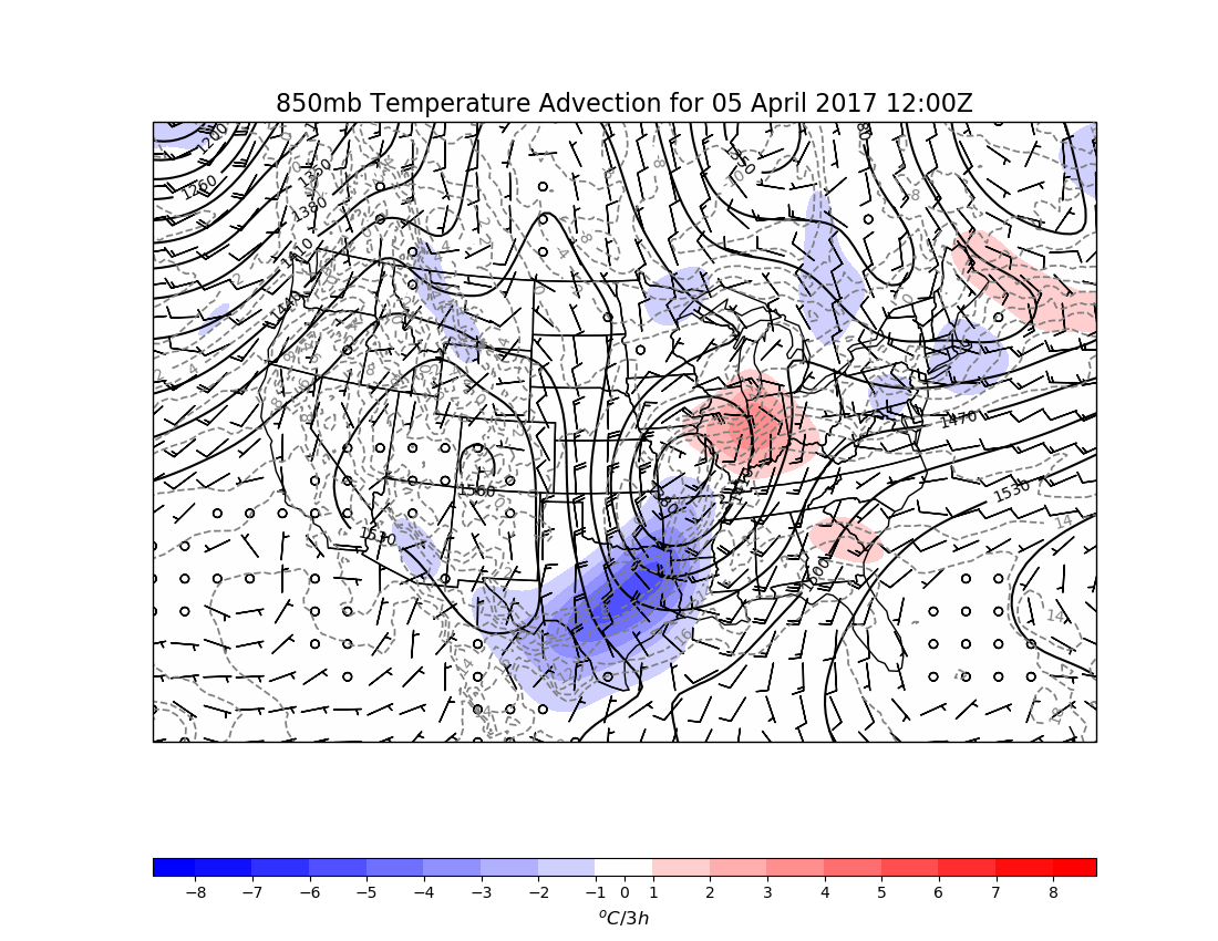
850 hPa Temperature Advection

Plot an 850 hPa map with calculating advection using MetPy.

Beyond just plotting 850-hPa level data, this uses calculations from metpy.calc to find the temperature advection. Currently, this needs an extra helper function to calculate the distance between lat/lon grid points.

Imports

from datetime import datetime

import cartopy.crs as ccrs
import cartopy.feature as cfeature
import matplotlib.gridspec as gridspec
import matplotlib.pyplot as plt
import metpy.calc as mpcalc
from metpy.units import units
from netCDF4 import num2date
import numpy as np
import scipy.ndimage as ndimage
from siphon.ncss import NCSS

Helper functions

# Helper function for finding proper time variable
def find_time_var(var, time_basename='time'):
    for coord_name in var.coordinates.split():
        if coord_name.startswith(time_basename):
            return coord_name
    raise ValueError('No time variable found for ' + var.name)

Create NCSS object to access the NetcdfSubset

Data from NCEI GFS 0.5 deg Analysis Archive

base_url = 'https://www.ncei.noaa.gov/thredds/ncss/grid/gfs-g4-anl-files/'
dt = datetime(2017, 4, 5, 12)
ncss = NCSS('{}{dt:%Y%m}/{dt:%Y%m%d}/gfsanl_4_{dt:%Y%m%d}_'
            '{dt:%H}00_000.grb2'.format(base_url, dt=dt))

# Create lat/lon box for location you want to get data for
query = ncss.query().time(dt)
query.lonlat_box(north=65, south=15, east=310, west=220)
query.accept('netcdf')

# Request data for vorticity
query.variables('Geopotential_height_isobaric', 'Temperature_isobaric',
                'u-component_of_wind_isobaric', 'v-component_of_wind_isobaric')
data = ncss.get_data(query)

# Pull out variables you want to use
hght_var = data.variables['Geopotential_height_isobaric']
temp_var = data.variables['Temperature_isobaric']
u_wind_var = data.variables['u-component_of_wind_isobaric']
v_wind_var = data.variables['v-component_of_wind_isobaric']
time_var = data.variables[find_time_var(temp_var)]
lat_var = data.variables['lat']
lon_var = data.variables['lon']

# Get actual data values and remove any size 1 dimensions
lat = lat_var[:].squeeze()
lon = lon_var[:].squeeze()
hght = hght_var[:].squeeze()
temp = temp_var[:].squeeze() * units.K
u_wind = units('m/s') * u_wind_var[:].squeeze()
v_wind = units('m/s') * v_wind_var[:].squeeze()

# Convert number of hours since the reference time into an actual date
time = num2date(time_var[:].squeeze(), time_var.units)

lev_850 = np.where(data.variables['isobaric'][:] == 850*100)[0][0]
hght_850 = hght[lev_850]
temp_850 = temp[lev_850]
u_wind_850 = u_wind[lev_850]
v_wind_850 = v_wind[lev_850]

# Combine 1D latitude and longitudes into a 2D grid of locations
lon_2d, lat_2d = np.meshgrid(lon, lat)
# Gridshift for barbs
lon_2d[lon_2d > 180] = lon_2d[lon_2d > 180] - 360

Begin data calculations

# Use helper function defined above to calculate distance
# between lat/lon grid points
dx, dy = mpcalc.lat_lon_grid_deltas(lon_var, lat_var)

# Calculate temperature advection using metpy function
adv = mpcalc.advection(temp_850 * units.kelvin, [u_wind_850, v_wind_850],
                       (dx, dy), dim_order='yx') * units('K/sec')

# Smooth heights and advection a little
# Be sure to only put in a 2D lat/lon or Y/X array for smoothing
Z_850 = ndimage.gaussian_filter(hght_850, sigma=3, order=0) * units.meter
adv = ndimage.gaussian_filter(adv, sigma=3, order=0) * units('K/sec')

Begin map creation

# Set Projection of Data
datacrs = ccrs.PlateCarree()

# Set Projection of Plot
plotcrs = ccrs.LambertConformal(central_latitude=[30, 60], central_longitude=-100)

# Create new figure
fig = plt.figure(figsize=(11, 8.5))
gs = gridspec.GridSpec(2, 1, height_ratios=[1, .02], bottom=.07, top=.99,
                       hspace=0.01, wspace=0.01)

# Add the map and set the extent
ax = plt.subplot(gs[0], projection=plotcrs)
plt.title('850mb Temperature Advection for {0:%d %B %Y %H:%MZ}'.format(time), fontsize=16)
ax.set_extent([235., 290., 20., 55.])

# Add state/country boundaries to plot
ax.add_feature(cfeature.STATES)
ax.add_feature(cfeature.BORDERS)

# Plot Height Contours
clev850 = np.arange(900, 3000, 30)
cs = ax.contour(lon_2d, lat_2d, Z_850, clev850, colors='black', linewidths=1.5,
                linestyles='solid', transform=datacrs)
plt.clabel(cs, fontsize=10, inline=1, inline_spacing=10, fmt='%i',
           rightside_up=True, use_clabeltext=True)

# Plot Temperature Contours
clevtemp850 = np.arange(-20, 20, 2)
cs2 = ax.contour(lon_2d, lat_2d, temp_850.to(units('degC')), clevtemp850,
                 colors='grey', linewidths=1.25, linestyles='dashed',
                 transform=datacrs)
plt.clabel(cs2, fontsize=10, inline=1, inline_spacing=10, fmt='%i',
           rightside_up=True, use_clabeltext=True)

# Plot Colorfill of Temperature Advection
cint = np.arange(-8, 9)
cf = ax.contourf(lon_2d, lat_2d, 3*adv.to(units('delta_degC/hour')), cint[cint != 0],
                 extend='both', cmap='bwr', transform=datacrs)
cax = plt.subplot(gs[1])
cb = plt.colorbar(cf, cax=cax, orientation='horizontal', extendrect=True, ticks=cint)
cb.set_label(r'$^{o}C/3h$', size='large')

# Plot Wind Barbs
ax.barbs(lon_2d, lat_2d, u_wind_850.magnitude, v_wind_850.magnitude,
         length=6, regrid_shape=20, pivot='middle', transform=datacrs)

plt.show()