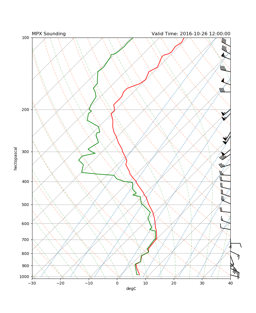
Skew-T Analysis

Classic skew-T/log-p plot using data from University of Wyoming.

This example uses example data from the University of Wyoming sounding archive for 12 UTC 31 October 2016 for Minneapolis, MN (MPX) and uses MetPy to plot the classic skew-T with Temperature, Dewpoint, and wind barbs.

from datetime import datetime

import matplotlib.pyplot as plt
from metpy.plots import SkewT
from metpy.units import pandas_dataframe_to_unit_arrays, units
import numpy as np
from siphon.simplewebservice.wyoming import WyomingUpperAir

Set time using a datetime object and station as variables

dt = datetime(2016, 10, 26, 12)
station = 'MPX'

Grab Remote Data

This requires an internet connection to access the sounding data from a remote server at the University of Wyoming.

# Read remote sounding data based on time (dt) and station
df = WyomingUpperAir.request_data(dt, station)

# Create dictionary of united arrays
data = pandas_dataframe_to_unit_arrays(df)

Isolate variables and attach units

# Isolate united arrays from dictionary to individual variables
p = data['pressure']
T = data['temperature']
Td = data['dewpoint']
u = data['u_wind']
v = data['v_wind']

Make Skew-T Plot

The code below makes a basic skew-T plot using the MetPy plot module that contains a SkewT class.

# Change default to be better for skew-T
fig = plt.figure(figsize=(9, 11))

# Initiate the skew-T plot type from MetPy class loaded earlier
skew = SkewT(fig, rotation=45)

# Plot the data using normal plotting functions, in this case using
# log scaling in Y, as dictated by the typical meteorological plot
skew.plot(p, T, 'r')
skew.plot(p, Td, 'g')
skew.plot_barbs(p[::3], u[::3], v[::3], y_clip_radius=0.03)

# Set some appropriate axes limits for x and y
skew.ax.set_xlim(-30, 40)
skew.ax.set_ylim(1020, 100)

# Add the relevant special lines to plot throughout the figure
skew.plot_dry_adiabats(t0=np.arange(233, 533, 10) * units.K,
                       alpha=0.25, color='orangered')
skew.plot_moist_adiabats(t0=np.arange(233, 400, 5) * units.K,
                         alpha=0.25, color='tab:green')
skew.plot_mixing_lines(p=np.arange(1000, 99, -20) * units.hPa,
                       linestyle='dotted', color='tab:blue')

# Add some descriptive titles
plt.title('{} Sounding'.format(station), loc='left')
plt.title('Valid Time: {}'.format(dt), loc='right')

plt.show()