Note
Click here to download the full example code
GOES-16: True Color Recipe
By: [Brian Blaylock](http://home.chpc.utah.edu/~u0553130/Brian_Blaylock/home.html) with help from Julien Chastang (UCAR-Unidata).
Additional notebooks analyzing GOES-16 and other data can be found in [Brian’s GitHub repository](https://github.com/blaylockbk/pyBKB_v3/).
This notebook shows how to make a true color image from the GOES-16 Advanced Baseline Imager (ABI) level 2 data. We will plot the image with matplotlib and Cartopy. The methods shown here are stitched together from the following online resources:
[CIMSS True Color RGB Quick Guide](http://cimss.ssec.wisc.edu/goes/OCLOFactSheetPDFs/ABIQuickGuide_CIMSSRGB_v2.pdf)
[ABI Bands Quick Information Guides](https://www.goes-r.gov/education/ABI-bands-quick-info.html)
[Open Commons Consortium](http://edc.occ-data.org/goes16/python/)
[GeoNetCast Blog](https://geonetcast.wordpress.com/2017/07/25/geonetclass-manipulating-goes-16-data-with-python-part-vi/)
[Proj documentation](https://proj4.org/operations/projections/geos.html?highlight=geostationary)
True color images are an RGB composite of the following three channels:
<table border=”1” class=”docutils”> <thead> <tr> <th>–</th> <th>Wavelength</th> <th>Channel</th> <th>Description</th> </tr> </thead> <tbody> <tr> <td><strong>Red</strong></td> <td>0.64 µm</td> <td>2</td> <td>Red Visible</td> </tr> <tr> <td><strong>Green</strong></td> <td>0.86 µm</td> <td>3</td> <td>Veggie Near-IR</td> </tr> <tr> <td><strong>Blue</strong></td> <td>0.47 µm</td> <td>1</td> <td>Blue Visible</td> </tr> </tbody> </table>
For this demo, we use the Level 2 Multichannel formated data (ABI-L2-MCMIP) for the CONUS domain. This file contains all sixteen channels on the ABI fixed grid (~2 km grid spacing).
GOES-16 data is downloaded from Unidata, but you may also download GOES-16 or 17 files from NOAA’s GOES archive on [Amazon S3](https://aws.amazon.com/public-datasets/goes/). I created a [web interface](http://home.chpc.utah.edu/~u0553130/Brian_Blaylock/cgi-bin/goes16_download.cgi?source=aws&satellite=noaa-goes16&domain=C&product=ABI-L2-MCMIP) to easily download files from the Amazon archive. For scripted or bulk downloads, you should use rclone or AWS CLI. You may also download files from the [Environmental Data Commons](http://edc.occ-data.org/goes16/getdata/) and [NOAA CLASS](https://www.avl.class.noaa.gov/saa/products/search?sub_id=0&datatype_family=GRABIPRD&submit.x=25&submit.y=9).
File names have the following format…
OR_ABI-L2-MCMIPC-M3_G16_s20181781922189_e20181781924562_c20181781925075.nc
OR - Indicates the system is operational
ABI - Instrument type
L2 - Level 2 Data
MCMIP - Multichannel Cloud and Moisture Imagery products
c - CONUS file (created every 5 minutes).
M3 - Scan mode
G16 - GOES-16
sYYYYJJJHHMMSSZ - Scan start: 4 digit year, 3 digit day of year (Julian day), hour, minute, second, tenth second
eYYYYJJJHHMMSSZ - Scan end
cYYYYJJJHHMMSSZ - File Creation .nc - NetCDF file extension
First, import the libraries we will use
from datetime import datetime

import cartopy.crs as ccrs
import matplotlib.pyplot as plt
import metpy  # noqa: F401
import numpy as np
import xarray
Open the GOES-16 NetCDF File
# Open the file with xarray.
# The opened file is assigned to "C" for the CONUS domain.

FILE = ('http://ramadda-jetstream.unidata.ucar.edu/repository/opendap'
        '/4ef52e10-a7da-4405-bff4-e48f68bb6ba2/entry.das#fillmismatch')
C = xarray.open_dataset(FILE)
Date and Time Information
Each file represents the data collected during one scan sequence for the domain. There are several different time stamps in this file, which are also found in the file’s name. I’m not a fan of numpy datetime, so I convert it to a regular datetime
# Scan's start time, converted to datetime object
scan_start = datetime.strptime(C.time_coverage_start, '%Y-%m-%dT%H:%M:%S.%fZ')

# Scan's end time, converted to datetime object
scan_end = datetime.strptime(C.time_coverage_end, '%Y-%m-%dT%H:%M:%S.%fZ')

# File creation time, convert to datetime object
file_created = datetime.strptime(C.date_created, '%Y-%m-%dT%H:%M:%S.%fZ')

# The 't' variable is the scan's midpoint time
midpoint = str(C['t'].data)[:-8]
scan_mid = datetime.strptime(midpoint, '%Y-%m-%dT%H:%M:%S.%f')

print('Scan Start    : {}'.format(scan_start))
print('Scan midpoint : {}'.format(scan_mid))
print('Scan End      : {}'.format(scan_end))
print('File Created  : {}'.format(file_created))
print('Scan Duration : {:.2f} minutes'.format((scan_end-scan_start).seconds/60))
Out:
Scan Start    : 2018-10-10 14:32:20.300000
Scan midpoint : 2018-10-10 14:33:38.900000
Scan End      : 2018-10-10 14:34:57.600000
File Created  : 2018-10-10 14:35:08.800000
Scan Duration : 2.62 minutes
True Color RGB Recipe
Color images are a Red-Green-Blue (RGB) composite of three different channels. To make a “Natural True Color” image we assign the following channels as our R, G, and B values:
<table border=”1” class=”docutils”> <thead> <tr> <th>–</th> <th>RED</th> <th>GREEN</th> <th>BLUE</th> </tr> </thead> <tbody> <tr> <td><strong>Name</strong></td> <td>Red Visible</td> <td>Near-IR Veggie</td> <td>Blue Visible</td> </tr> <tr> <td><strong>Wavelength</strong></td> <td>0.64 µm</td> <td>0.86 µm</td> <td>0.47 µm</td> </tr> <tr> <td><strong>Channel</strong></td> <td>2</td> <td>3</td> <td>1</td> </tr> <tr> <td><strong>Units</strong></td> <td>Reflectance</td> <td>Reflectance</td> <td>Reflectance</td> </tr> <tr> <td><strong>Range of Values</strong></td> <td>0-1</td> <td>0-1</td> <td>0-1</td> </tr> <tr> <td><strong>Gamma Correction</strong></td> <td>2.2</td> <td>2.2</td> <td>2.2</td> </tr> </tbody> </table>
Some important details to know about…
Value Range: The data units of channel 1, 2, and 3 are in reflectance and have a range of values between 0 and 1. RGB values must also be between 0 and 1.
Gamma Correction: A gamma correction is applied to control the brightness and make the image not look too dark. corrected_value = value^(1/gamma). Most displays have a decoding gamma of 2.2. Read more about gamma correction at the following links… [source1](https://en.wikipedia.org/wiki/Gamma_correction) and [source2](https://www.cambridgeincolour.com/tutorials/gamma-correction.htm)).
True Green: The GREEN “veggie” channel on GOES-16 does not measure visible green light. Instead, it measures a near-infrared band sensitive to chlorophyll. We could use that channel in place of green, but it would make the green in our image appear too vibrant. Instead, we will tone-down the green channel by interpolating the value to simulate a natural green color.
TrueGreen = (0.45*RED) + (0.1*GREEN) + (0.45*BLUE)
Now we can begin putting the pieces together…
# Confirm that each band is the wavelength we are interested in
for band in [2, 3, 1]:
    print('{} is {:.2f} {}'.format(
        C['band_wavelength_C{:02d}'.format(band)].long_name,
        float(C['band_wavelength_C{:02d}'.format(band)][0]),
        C['band_wavelength_C{:02d}'.format(band)].units))
Out:
ABI band 2 central wavelength is 0.64 um
ABI band 3 central wavelength is 0.87 um
ABI band 1 central wavelength is 0.47 um
Simple Image
Use plt.imshow to get a quick look at the channels and RGB composite we created.
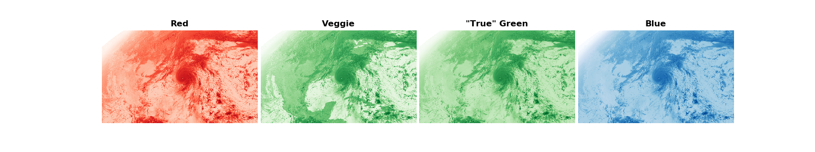
First, plot each channel individually. The deeper the color means the satellite is observing more light in that channel. Clouds appear white because they reflect lots of red, green, and blue light. Notice that the land reflects a lot of “green” in the veggie channel because this channel is sensitive to the chlorophyll.
fig, ([ax1, ax2, ax3, ax4]) = plt.subplots(1, 4, figsize=(16, 3))
ax1.imshow(R, cmap='Reds', vmax=1, vmin=0)
ax1.set_title('Red', fontweight='bold')
ax1.axis('off')
ax2.imshow(G, cmap='Greens', vmax=1, vmin=0)
ax2.set_title('Veggie', fontweight='bold')
ax2.axis('off')
ax3.imshow(G_true, cmap='Greens', vmax=1, vmin=0)
ax3.set_title('"True" Green', fontweight='bold')
ax3.axis('off')
ax4.imshow(B, cmap='Blues', vmax=1, vmin=0)
ax4.set_title('Blue', fontweight='bold')
ax4.axis('off')
plt.subplots_adjust(wspace=.02)
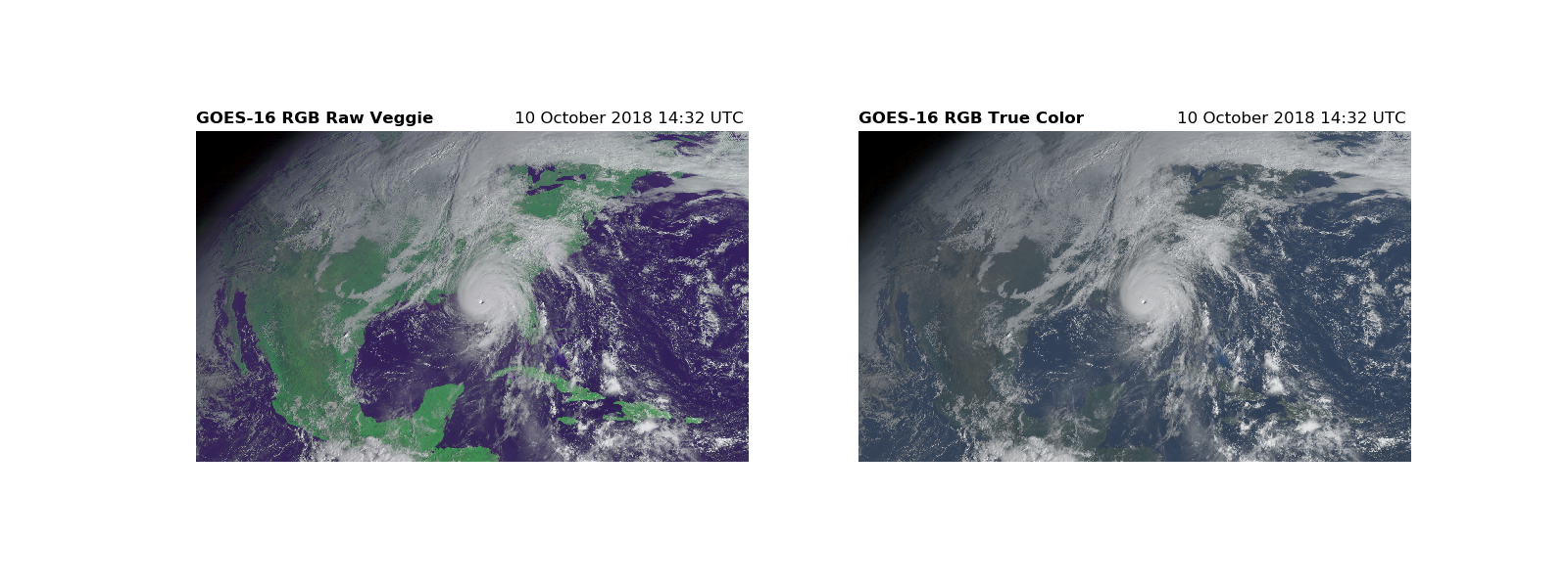
The addition of the three channels results in a color image. Combine the three channels with a stacked array and display the image with imshow.
# The RGB array with the raw veggie band
RGB_veggie = np.dstack([R, G, B])
# The RGB array for the true color image
RGB = np.dstack([R, G_true, B])
fig, (ax1, ax2) = plt.subplots(1, 2, figsize=(16, 6))
# The RGB using the raw veggie band
ax1.imshow(RGB_veggie)
ax1.set_title('GOES-16 RGB Raw Veggie', fontweight='bold', loc='left',
fontsize=12)
ax1.set_title('{}'.format(scan_start.strftime('%d %B %Y %H:%M UTC ')),
loc='right')
ax1.axis('off')
# The RGB for the true color image
ax2.imshow(RGB)
ax2.set_title('GOES-16 RGB True Color', fontweight='bold', loc='left',
fontsize=12)
ax2.set_title('{}'.format(scan_start.strftime('%d %B %Y %H:%M UTC ')),
loc='right')
ax2.axis('off')
Out:
(-0.5, 2499.5, 1499.5, -0.5)
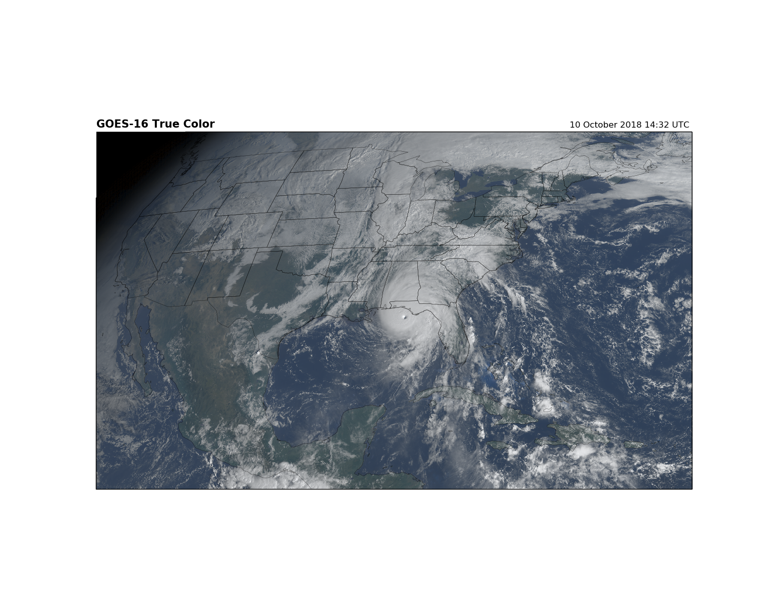
Plot with Cartopy Geostationary Projection
The image above is not georeferenced. You can see the land and oceans, but we do have enough information to draw state and country boundaries. Use the metpy.io package to obtain the projection information from the file. Then use Cartopy to plot the image on a map. The GOES data and image is on a [geostationary projection ](https://proj4.org/operations/projections/geos.html?highlight=geostationary).
# We'll use the `CMI_C02` variable as a 'hook' to get the CF metadata.
dat = C.metpy.parse_cf('CMI_C02')
geos = dat.metpy.cartopy_crs
# We also need the x (north/south) and y (east/west) axis sweep of the ABI data
x = dat.x
y = dat.y
The geostationary projection is the easiest way to plot the image on a map. Essentially, we are stretching the image across a map with the same projection and dimensions as the data.
fig = plt.figure(figsize=(15, 12))
# Create axis with Geostationary projection
ax = fig.add_subplot(1, 1, 1, projection=geos)
# Add the RGB image to the figure. The data is in the same projection as the
# axis we just created.
ax.imshow(RGB, origin='upper',
extent=(x.min(), x.max(), y.min(), y.max()), transform=geos)
# Add Coastlines and States
ax.coastlines(resolution='50m', color='black', linewidth=0.25)
ax.add_feature(ccrs.cartopy.feature.STATES, linewidth=0.25)
plt.title('GOES-16 True Color', loc='left', fontweight='bold', fontsize=15)
plt.title('{}'.format(scan_start.strftime('%d %B %Y %H:%M UTC ')), loc='right')
plt.show()
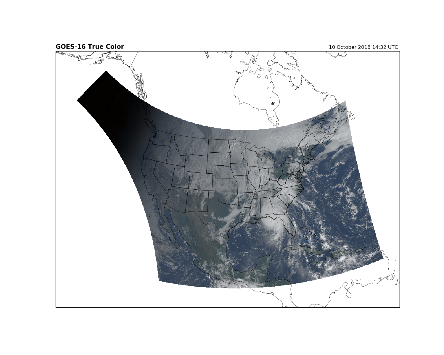
Using other projections
Changing the projections with Cartopy is straightforward. Here we display the GOES-16 data on a Lambert Conformal projection.
fig = plt.figure(figsize=(15, 12))
# Generate an Cartopy projection
lc = ccrs.LambertConformal(central_longitude=-97.5, standard_parallels=(38.5,
38.5))
ax = fig.add_subplot(1, 1, 1, projection=lc)
ax.set_extent([-135, -60, 10, 65], crs=ccrs.PlateCarree())
ax.imshow(RGB, origin='upper',
extent=(x.min(), x.max(), y.min(), y.max()),
transform=geos,
interpolation='none')
ax.coastlines(resolution='50m', color='black', linewidth=0.5)
ax.add_feature(ccrs.cartopy.feature.STATES, linewidth=0.5)
plt.title('GOES-16 True Color', loc='left', fontweight='bold', fontsize=15)
plt.title('{}'.format(scan_start.strftime('%d %B %Y %H:%M UTC ')), loc='right')
plt.show()
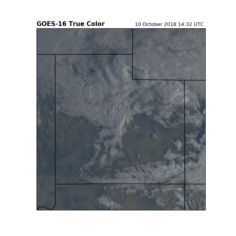
Plot with Cartopy: Plate Carrée Cylindrical Projection
It is often useful to zoom on a specific location. This image will zoom in on Utah.
fig = plt.figure(figsize=(8, 8))
pc = ccrs.PlateCarree()
ax = fig.add_subplot(1, 1, 1, projection=pc)
ax.set_extent([-114.75, -108.25, 36, 43], crs=pc)
ax.imshow(RGB, origin='upper',
extent=(x.min(), x.max(), y.min(), y.max()),
transform=geos,
interpolation='none')
ax.coastlines(resolution='50m', color='black', linewidth=1)
ax.add_feature(ccrs.cartopy.feature.STATES)
plt.title('GOES-16 True Color', loc='left', fontweight='bold', fontsize=15)
plt.title('{}'.format(scan_start.strftime('%d %B %Y %H:%M UTC ')), loc='right')
plt.show()
Overlay Nighttime IR when dark
At nighttime, the visible wavelengths do not measure anything and is just black. There is information, however, from other channels we can use to see clouds at night. To view clouds in portions of the domain experiencing nighttime, we will overlay the clean infrared (IR) channel over the true color image.
First, open a file where the scan shows partial night area and create the true color RGB as before.
# A GOES-16 file with half day and half night
FILE = ('http://ramadda-jetstream.unidata.ucar.edu/repository/opendap'
'/85da3304-b910-472b-aedf-a6d8c1148131/entry.das#fillmismatch')
C = xarray.open_dataset(FILE)
# Scan's start time, converted to datetime object
scan_start = datetime.strptime(C.time_coverage_start, '%Y-%m-%dT%H:%M:%S.%fZ')
# Create the RGB like we did before
# Load the three channels into appropriate R, G, and B
R = C['CMI_C02'].data
G = C['CMI_C03'].data
B = C['CMI_C01'].data
# Apply range limits for each channel. RGB values must be between 0 and 1
R = np.clip(R, 0, 1)
G = np.clip(G, 0, 1)
B = np.clip(B, 0, 1)
# Apply the gamma correction
gamma = 2.2
R = np.power(R, 1/gamma)
G = np.power(G, 1/gamma)
B = np.power(B, 1/gamma)
# Calculate the "True" Green
G_true = 0.45 * R + 0.1 * G + 0.45 * B
G_true = np.clip(G_true, 0, 1)
# The final RGB array :)
RGB = np.dstack([R, G_true, B])
Load the Clear IR 10.3 µm channel (Band 13)
When you print the contents of channel 13, notice that the unit of the clean IR channel is brightness temperature, NOT reflectance. We need to normalize the values between 0 and 1 before we can use it in our RGB image. In this case, we normalize the values between 90 Kelvin and 313 Kelvin.
print(C['CMI_C13'])
Out:
<xarray.DataArray 'CMI_C13' (y: 1500, x: 2500)>
[3750000 values with dtype=float32]
Coordinates:
    t        datetime64[ns] ...
  * y        (y) float32 0.128212 0.128156 ... 0.044324003 0.044268005
  * x        (x) float32 -0.101332 -0.101276 ... 0.038556002 0.038612
    y_image  float32 ...
    x_image  float32 ...
Attributes:
    long_name:              ABI Cloud and Moisture Imagery brightness tempera...
    standard_name:          toa_brightness_temperature
    sensor_band_bit_depth:  12
    valid_range:            [   0 4095]
    units:                  K
    resolution:             y: 0.000056 rad x: 0.000056 rad
    grid_mapping:           goes_imager_projection
    cell_methods:           t: point area: point
    ancillary_variables:    DQF_C13
    _ChunkSizes:            [250 250]
Apply the normalization…
cleanIR = C['CMI_C13'].data

# Normalize the channel between a range.
#       cleanIR = (cleanIR-minimumValue)/(maximumValue-minimumValue)
cleanIR = (cleanIR-90)/(313-90)

# Apply range limits to make sure values are between 0 and 1
cleanIR = np.clip(cleanIR, 0, 1)

# Invert colors so that cold clouds are white
cleanIR = 1 - cleanIR

# Lessen the brightness of the coldest clouds so they don't appear so bright
# when we overlay it on the true color image.
cleanIR = cleanIR/1.4

# Yes, we still need 3 channels as RGB values. This will be a grey image.
RGB_cleanIR = np.dstack([cleanIR, cleanIR, cleanIR])
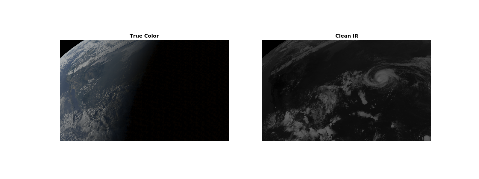
Show the true color and clean IR images
We want to overlay these two images, so the clean IR fills in the night sky on the True Color image. This way we can still see the clouds at night.
fig, (ax1, ax2) = plt.subplots(1, 2, figsize=(16, 6))

ax1.set_title('True Color', fontweight='bold')
ax1.imshow(RGB)
ax1.axis('off')

ax2.set_title('Clean IR', fontweight='bold')
ax2.imshow(RGB_cleanIR)
ax2.axis('off')

plt.show()
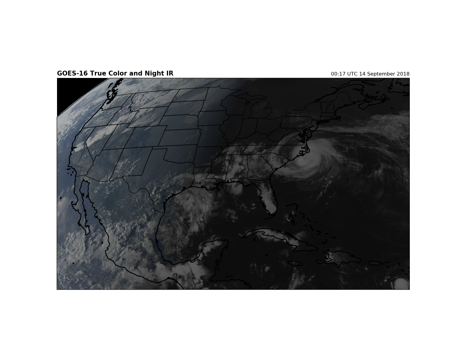
To fill in the dark area on the true color image, we will set each RGB channel to equal the maximum value between the visible channels and the IR channels. When this is done, where RGB values are black in the true color image RGB = (0,0,0), it will be replaced with a higher value of the cleanIR RGB.
Note that if the clean IR has really bright, cold clouds in the daylight, they will replace the color values in the true color image making the clouds appear more white. Still, it makes a nice plot and let’s you see clouds when it is night.
# Maximize the RGB values between the True Color Image and Clean IR image
RGB_ColorIR = np.dstack([np.maximum(R, cleanIR), np.maximum(G_true, cleanIR),
                         np.maximum(B, cleanIR)])
fig = plt.figure(figsize=(15, 12))

ax = fig.add_subplot(1, 1, 1, projection=geos)

ax.imshow(RGB_ColorIR, origin='upper',
          extent=(x.min(), x.max(), y.min(), y.max()),
          transform=geos)

ax.coastlines(resolution='50m', color='black', linewidth=2)
ax.add_feature(ccrs.cartopy.feature.STATES)

plt.title('GOES-16 True Color and Night IR', loc='left', fontweight='bold',
          fontsize=15)
plt.title('{}'.format(scan_start.strftime('%H:%M UTC %d %B %Y'), loc='right'),
          loc='right')

plt.show()
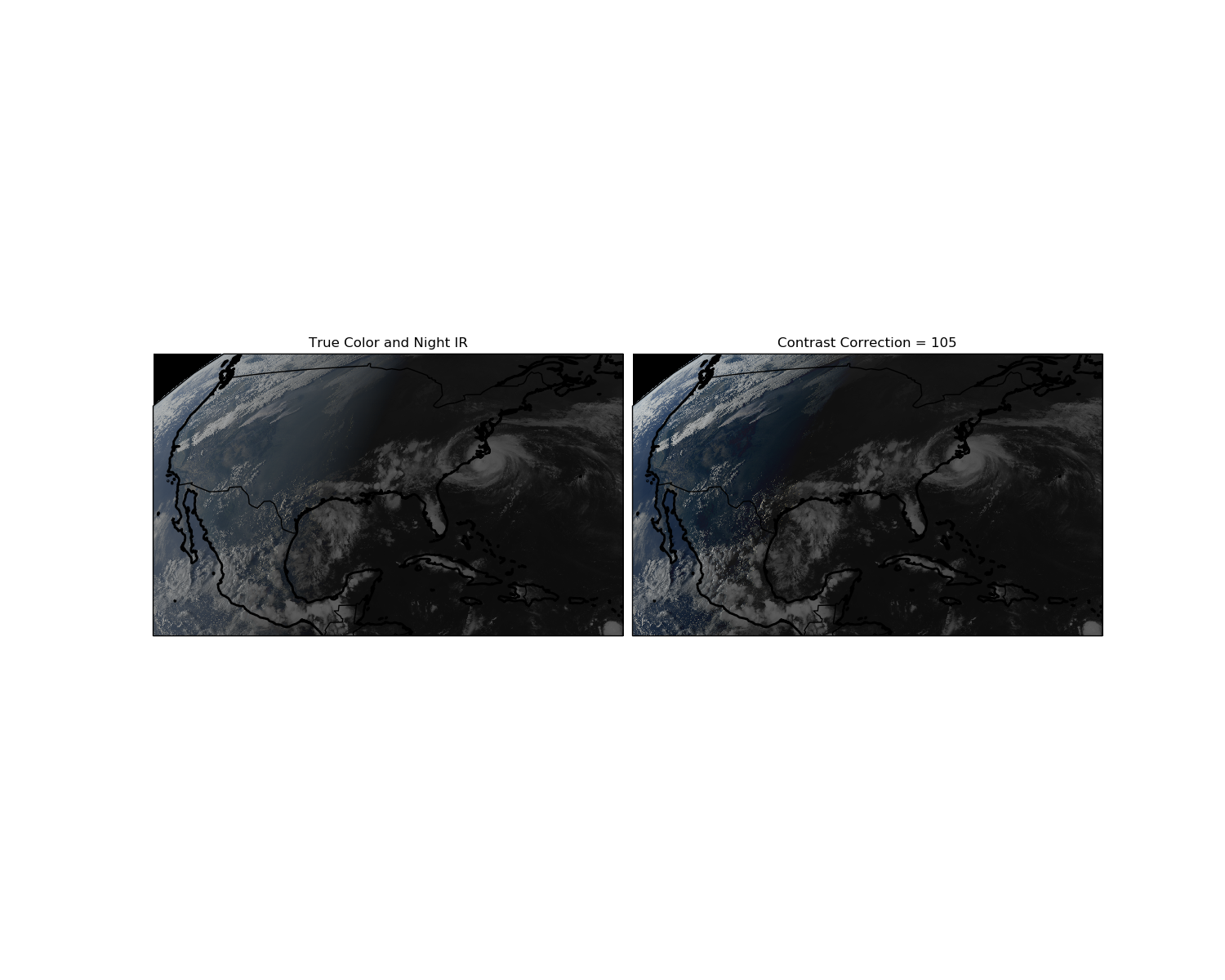
Adjust Image Contrast
I think the color looks a little dull. We could get complicated and make a Rayleigh correction to the data to fix the blue light scattering, but that can be intense. More simply, we can make the colors pop out by adjusting the image contrast. Adjusting image contrast is easy to do in Photoshop, and also easy to do in Python.
We are still using the RGB values from the day/night GOES-16 ABI scan.
Note: you should adjust the contrast _before_ you add in the Clean IR channel.
def contrast_correction(color, contrast):
    """
    Modify the contrast of an RGB
    See:
    https://www.dfstudios.co.uk/articles/programming/image-programming-algorithms/image-processing-algorithms-part-5-contrast-adjustment/

    Input:
        color    - an array representing the R, G, and/or B channel
        contrast - contrast correction level
    """
    F = (259*(contrast + 255))/(255.*259-contrast)
    COLOR = F*(color-.5)+.5
    COLOR = np.clip(COLOR, 0, 1)  # Force value limits 0 through 1.
    return COLOR

# Amount of contrast
contrast_amount = 105

# Apply contrast correction
RGB_contrast = contrast_correction(RGB, contrast_amount)

# Add in clean IR to the contrast-corrected True Color image
RGB_contrast_IR = np.dstack([np.maximum(RGB_contrast[:, :, 0], cleanIR),
                             np.maximum(RGB_contrast[:, :, 1], cleanIR),
                             np.maximum(RGB_contrast[:, :, 2], cleanIR)])
# Plot on map with Cartopy

fig = plt.figure(figsize=(15, 12))

ax1 = fig.add_subplot(1, 2, 1, projection=geos)
ax2 = fig.add_subplot(1, 2, 2, projection=geos)

ax1.imshow(RGB_ColorIR, origin='upper',
           extent=(x.min(), x.max(), y.min(), y.max()),
           transform=geos)
ax1.coastlines(resolution='50m', color='black', linewidth=2)
ax1.add_feature(ccrs.cartopy.feature.BORDERS)
ax1.set_title('True Color and Night IR')

ax2.imshow(RGB_contrast_IR, origin='upper',
           extent=(x.min(), x.max(), y.min(), y.max()),
           transform=geos)
ax2.coastlines(resolution='50m', color='black', linewidth=2)
ax2.add_feature(ccrs.cartopy.feature.BORDERS)
ax2.set_title('Contrast Correction = {}'.format(contrast_amount))

plt.subplots_adjust(wspace=.02)
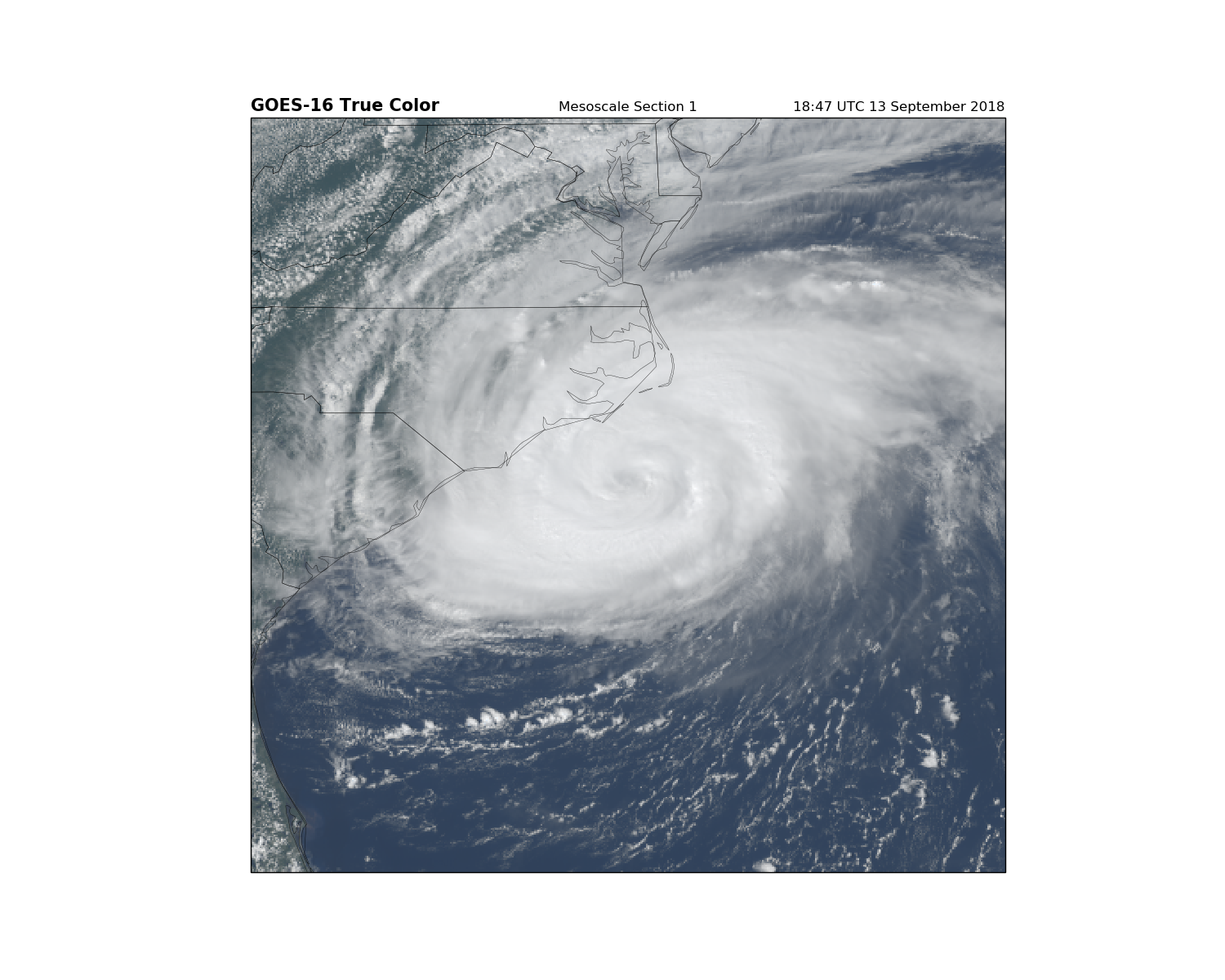
Can we make plots for a Mesoscale scan?
Yes. Yes we can.
# M1 is for the Mesoscale1 NetCDF file

FILE = ('http://ramadda-jetstream.unidata.ucar.edu/repository/opendap'
        '/5e02eafa-5cee-4d00-9f58-6e201e69b014/entry.das#fillmismatch')
M1 = xarray.open_dataset(FILE)

# Load the RGB arrays
R = M1['CMI_C02'][:].data
G = M1['CMI_C03'][:].data
B = M1['CMI_C01'][:].data

# Apply range limits for each channel. RGB values must be between 0 and 1
R = np.clip(R, 0, 1)
G = np.clip(G, 0, 1)
B = np.clip(B, 0, 1)

# Apply the gamma correction
gamma = 2.2
R = np.power(R, 1/gamma)
G = np.power(G, 1/gamma)
B = np.power(B, 1/gamma)

# Calculate the "True" Green
G_true = 0.45 * R + 0.1 * G + 0.45 * B
G_true = np.clip(G_true, 0, 1)

# The final RGB array :)
RGB = np.dstack([R, G_true, B])

# Scan's start time, converted to datetime object
scan_start = datetime.strptime(M1.time_coverage_start, '%Y-%m-%dT%H:%M:%S.%fZ')

# We'll use the `CMI_C02` variable as a 'hook' to get the CF metadata.
dat = M1.metpy.parse_cf('CMI_C02')

# Need the satellite sweep x and y values, too.
x = dat.x
y = dat.y
fig = plt.figure(figsize=(10, 8))

ax = fig.add_subplot(1, 1, 1, projection=lc)
ax.set_extent([-125, -70, 25, 50], crs=ccrs.PlateCarree())

ax.imshow(RGB, origin='upper',
          extent=(x.min(), x.max(), y.min(), y.max()),
          transform=geos)

ax.coastlines(resolution='50m', color='black', linewidth=0.5)
ax.add_feature(ccrs.cartopy.feature.STATES, linewidth=0.5)
ax.add_feature(ccrs.cartopy.feature.BORDERS, linewidth=0.5)

plt.title('GOES-16 True Color', fontweight='bold', fontsize=15, loc='left')
plt.title('Mesoscale Section 1')
plt.title('{}'.format(scan_start.strftime('%H:%M UTC %d %B %Y')), loc='right')

plt.show()
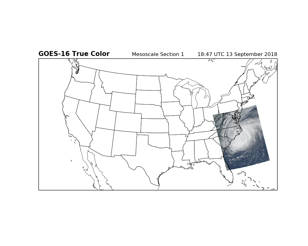
fig = plt.figure(figsize=(15, 12))

ax = fig.add_subplot(1, 1, 1, projection=geos)

ax.imshow(RGB, origin='upper',
          extent=(x.min(), x.max(), y.min(), y.max()),
          transform=geos)

ax.coastlines(resolution='50m', color='black', linewidth=0.25)
ax.add_feature(ccrs.cartopy.feature.STATES, linewidth=0.25)

plt.title('GOES-16 True Color', fontweight='bold', fontsize=15, loc='left')
plt.title('Mesoscale Section 1')
plt.title('{}'.format(scan_start.strftime('%H:%M UTC %d %B %Y')), loc='right')

plt.show()
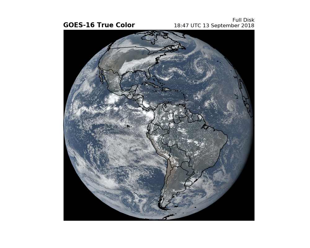
Can we do this for a Full Disk Scan? It’s possible…
but data files are so large that plotting is very slow. Feel free to experiment.
FILE = ('http://ramadda-jetstream.unidata.ucar.edu/repository/opendap'
        '/deb91f58-f997-41a3-a077-987529bf02b3/entry.das#fillmismatch')
F = xarray.open_dataset(FILE)

# Load the RGB arrays
R = F['CMI_C02'][:].data
G = F['CMI_C03'][:].data
B = F['CMI_C01'][:].data

# Apply range limits for each channel. RGB values must be between 0 and 1
R = np.clip(R, 0, 1)
G = np.clip(G, 0, 1)
B = np.clip(B, 0, 1)

# Apply the gamma correction
gamma = 2.2
R = np.power(R, 1/gamma)
G = np.power(G, 1/gamma)
B = np.power(B, 1/gamma)

# Calculate the "True" Green
G_true = 0.48358168 * R + 0.45706946 * B + 0.06038137 * G
G_true = np.clip(G_true, 0, 1)

# The final RGB array :)
RGB = np.dstack([R, G_true, B])

# We'll use the `CMI_C02` variable as a 'hook' to get the CF metadata.
dat = F.metpy.parse_cf('CMI_C02')

x = dat.x
y = dat.y
Geostationary projection is easy…
fig = plt.figure(figsize=(10, 8))

ax = fig.add_subplot(1, 1, 1, projection=geos)

ax.imshow(RGB, origin='upper',
          extent=(x.min(), x.max(), y.min(), y.max()),
          transform=geos)

ax.coastlines(resolution='50m', color='black', linewidth=1)
ax.add_feature(ccrs.cartopy.feature.BORDERS, linewidth=1)

plt.title('GOES-16 True Color', fontweight='bold', fontsize=15, loc='left')
plt.title('Full Disk\n{}'.format(scan_start.strftime('%H:%M UTC %d %B %Y')),
          loc='right')

plt.show()
Total running time of the script: ( 0 minutes 44.406 seconds)