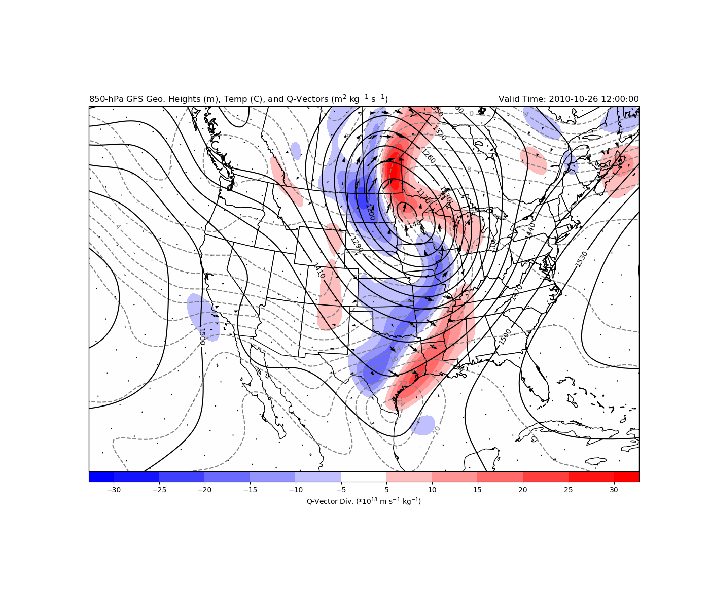
QVector Example

Computing Q-vectors and Q-vector divergence for a real case.

By: Kevin Goebbert

This example uses GFS output to compute the 850-hPa Q-vectors and Q-vector divergence for 12 UTC 26 October 2010.

Import needed modules

import cartopy.crs as ccrs
import cartopy.feature as cfeature
import matplotlib.pyplot as plt
import metpy.calc as mpcalc
from metpy.units import units
import numpy as np
import xarray as xr

Use Xarray to access GFS data from THREDDS resource and uses metpy accessor to parse file to make it easy to pull data using common coordinate names (e.g., vertical) and attach units.

ds = xr.open_dataset('https://thredds.ucar.edu/thredds/dodsC/casestudies/'
                     'python-gallery/GFS_20101026_1200.nc').metpy.parse_cf()

Subset data based on latitude and longitude values and select only data from 850 hPa

# Set subset slice for the geographic extent of data to limit download
lon_slice = slice(200, 350)
lat_slice = slice(85, 10)

# Grab lat/lon values (GFS will be 1D)
lats = ds.lat.sel(lat=lat_slice).values
lons = ds.lon.sel(lon=lon_slice).values

# Grab data and smooth using a nine-point filter applied 50 times to grab the synoptic signal
level = 850 * units.hPa
hght_850 = mpcalc.smooth_n_point(ds.Geopotential_height_isobaric.metpy.sel(
    vertical=level, lat=lat_slice, lon=lon_slice).squeeze(), 9, 50)
tmpk_850 = mpcalc.smooth_n_point(ds.Temperature_isobaric.metpy.sel(
    vertical=level, lat=lat_slice, lon=lon_slice).squeeze(), 9, 25)
uwnd_850 = mpcalc.smooth_n_point(ds['u-component_of_wind_isobaric'].metpy.sel(
    vertical=level, lat=lat_slice, lon=lon_slice).squeeze(), 9, 50)
vwnd_850 = mpcalc.smooth_n_point(ds['v-component_of_wind_isobaric'].metpy.sel(
    vertical=level, lat=lat_slice, lon=lon_slice).squeeze(), 9, 50)

# Convert temperatures to degree Celsius for plotting purposes
tmpc_850 = tmpk_850.to('degC')

# Get a sensible datetime format
vtime = ds.time.data[0].astype('datetime64[ms]').astype('O')

Compute Q-vectors

Use the MetPy module to compute Q-vectors from requisite data and additionally compute the Q-vector divergence (and multiply by -2) to calculate the right hand side forcing of the Q-G Omega equation.

# Compute grid spacings for data
dx, dy = mpcalc.lat_lon_grid_deltas(lons, lats)

# Compute the Q-vector components
uqvect, vqvect = mpcalc.q_vector(uwnd_850, vwnd_850, tmpk_850, 850*units.hPa, dx, dy)

# Compute the divergence of the Q-vectors calculated above
q_div = -2*mpcalc.divergence(uqvect, vqvect, dx, dy, dim_order='yx')

Plot Data

Use Cartopy to plot data on a map using a Lambert Conformal projection.

# Set the map projection (how the data will be displayed)
mapcrs = ccrs.LambertConformal(
    central_longitude=-100, central_latitude=35, standard_parallels=(30, 60))

# Set the data project (GFS is lat/lon format)
datacrs = ccrs.PlateCarree()

# Start the figure and set an extent to only display a smaller graphics area
fig = plt.figure(1, figsize=(14, 12))
ax = plt.subplot(111, projection=mapcrs)
ax.set_extent([-130, -72, 20, 55], ccrs.PlateCarree())

# Add map features to plot coastlines and state boundaries
ax.add_feature(cfeature.COASTLINE.with_scale('50m'))
ax.add_feature(cfeature.STATES.with_scale('50m'))

# Plot 850-hPa Q-Vector Divergence and scale
clevs_850_tmpc = np.arange(-40, 41, 2)
clevs_qdiv = list(range(-30, -4, 5))+list(range(5, 31, 5))
cf = ax.contourf(lons, lats, q_div*1e18, clevs_qdiv, cmap=plt.cm.bwr,
                 extend='both', transform=datacrs)
cb = plt.colorbar(cf, orientation='horizontal', pad=0, aspect=50, extendrect=True,
                  ticks=clevs_qdiv)
cb.set_label('Q-Vector Div. (*10$^{18}$ m s$^{-1}$ kg$^{-1}$)')

# Plot 850-hPa Temperatures
csf = ax.contour(lons, lats, tmpc_850, clevs_850_tmpc, colors='grey',
                 linestyles='dashed', transform=datacrs)
plt.clabel(csf, fmt='%d')

# Plot 850-hPa Geopotential Heights
clevs_850_hght = np.arange(0, 8000, 30)
cs = ax.contour(lons, lats, hght_850, clevs_850_hght, colors='black', transform=datacrs)
plt.clabel(cs, fmt='%d')

# Plot 850-hPa Q-vectors, scale to get nice sized arrows
wind_slice = (slice(None, None, 5), slice(None, None, 5))
ax.quiver(lons[wind_slice[0]], lats[wind_slice[1]],
          uqvect[wind_slice].m,
          vqvect[wind_slice].m,
          pivot='mid', color='black',
          scale=1e-11, scale_units='inches',
          transform=datacrs)

# Add some titles
plt.title('850-hPa GFS Geo. Heights (m), Temp (C),'
          ' and Q-Vectors (m$^2$ kg$^{-1}$ s$^{-1}$)', loc='left')
plt.title('Valid Time: {}'.format(vtime), loc='right')

plt.show()