NCSS Time Series

Use Siphon to query the NetCDF Subset Service for a timeseries.

from datetime import datetime, timedelta

import matplotlib.pyplot as plt
from netCDF4 import num2date

from siphon.catalog import TDSCatalog

First we construct a TDSCatalog instance pointing to our dataset of interest, in this case TDS’ “Best” virtual dataset for the GFS global 0.5 degree collection of GRIB files. We see this catalog contains a single dataset.

best_gfs = TDSCatalog('http://thredds.ucar.edu/thredds/catalog/grib/NCEP/GFS/'
                      'Global_0p5deg/catalog.xml?dataset=grib/NCEP/GFS/Global_0p5deg/Best')
print(best_gfs.datasets)

Out:

['Best GFS Half Degree Forecast Time Series']

We pull out this dataset and get the NCSS access point

best_ds = best_gfs.datasets[0]
ncss = best_ds.subset()

We can then use the ncss object to create a new query object, which facilitates asking for data from the server.

query = ncss.query()

We construct a query asking for data corresponding to latitude 40N and longitude 105W, for the next 7 days. We also ask for NetCDF version 4 data, for the variable ‘Temperature_isobaric’, at the vertical level of 100000 Pa (approximately surface). This request will return all times in the range for a single point. Note the string representation of the query is a properly encoded query string.

now = datetime.utcnow()
query.lonlat_point(-105, 40).vertical_level(100000).time_range(now, now + timedelta(days=7))
query.variables('Temperature_isobaric').accept('netcdf')

We now request data from the server using this query. The NCSS class handles parsing this NetCDF data (using the netCDF4 module). If we print out the variable names, we see our requested variables, as well as a few others (more metadata information)

data = ncss.get_data(query)
list(data.variables)

We’ll pull out the temperature and time variables.

temp = data.variables['Temperature_isobaric']
time = data.variables['time']

The time values are in hours relative to the start of the entire model collection. Fortunately, the netCDF4 module has a helper function to convert these numbers into Python datetime objects. We can see the first 5 element output by the function look reasonable.

time_vals = num2date(time[:].squeeze(), time.units)
print(time_vals[:5])

Out:

[datetime.datetime(2018, 8, 15, 0, 0) datetime.datetime(2018, 8, 15, 3, 0)
 datetime.datetime(2018, 8, 15, 6, 0) datetime.datetime(2018, 8, 15, 9, 0)
 datetime.datetime(2018, 8, 15, 12, 0)]

Now we can plot these up using matplotlib, which has ready-made support for datetime objects.

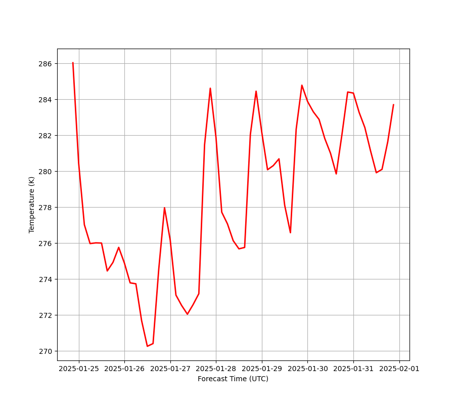
fig, ax = plt.subplots(1, 1, figsize=(9, 8))
ax.plot(time_vals, temp[:].squeeze(), 'r', linewidth=2)
ax.set_ylabel('{} ({})'.format(temp.standard_name, temp.units))
ax.set_xlabel('Forecast Time (UTC)')
ax.grid(True)

Total running time of the script: ( 0 minutes 1.749 seconds)