Basic NCSS

Use Siphon to query the NetCDF Subset Service (NCSS).

from datetime import datetime

import matplotlib.pyplot as plt

from siphon.catalog import TDSCatalog

First we construct a TDSCatalog instance pointing to our dataset of interest, in this case TDS’ “Best” virtual dataset for the GFS global 0.5 degree collection of GRIB files. We see this catalog contains a single dataset.

best_gfs = TDSCatalog('http://thredds.ucar.edu/thredds/catalog/grib/NCEP/GFS/'
                      'Global_0p5deg/catalog.xml?dataset=grib/NCEP/GFS/Global_0p5deg/Best')
print(best_gfs.datasets)

Out:

['Best GFS Half Degree Forecast Time Series']

We pull out this dataset and get the NCSS access point

best_ds = best_gfs.datasets[0]
ncss = best_ds.subset()

We can then use the ncss object to create a new query object, which facilitates asking for data from the server.

query = ncss.query()

We construct a query asking for data corresponding to latitude 40N and longitude 105W, for the current time. We also ask for NetCDF version 4 data, for the variables ‘Temperature_isobaric’ and ‘Relative_humidity_isobaric’. This request will return all vertical levels for a single point and single time. Note the string representation of the query is a properly encoded query string.

query.lonlat_point(-105, 40).time(datetime.utcnow())
query.accept('netcdf4')
query.variables('Temperature_isobaric', 'Relative_humidity_isobaric')

We now request data from the server using this query. The NCSS class handles parsing this NetCDF data (using the netCDF4 module). If we print out the variable names, we see our requested variables, as well as a few others (more metadata information)

data = ncss.get_data(query)
list(data.variables)

We’ll pull out the variables we want to use, as well as the pressure values. To get the name of the correct variable for pressure (which matches the levels for temperature and relative humidity, we look at the coordinates attribute. The last of the variables listed in coordinates is the pressure dimension.

temp = data.variables['Temperature_isobaric']
relh = data.variables['Relative_humidity_isobaric']
press_name = relh.coordinates.split()[-1]
press = data.variables[press_name]
press_vals = press[:].squeeze()

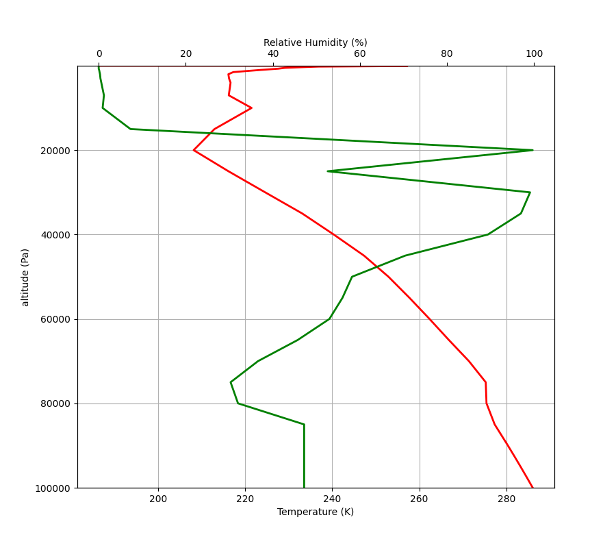
Now we can plot these up using matplotlib.

fig, ax = plt.subplots(1, 1, figsize=(9, 8))
ax.plot(temp[:].squeeze(), press_vals, 'r', linewidth=2)
ax.set_xlabel('{} ({})'.format(temp.standard_name, temp.units))
ax.set_ylabel('{} ({})'.format(press.standard_name, press.units))

# Create second plot with shared y-axis
ax2 = plt.twiny(ax)
ax2.plot(relh[:].squeeze(), press_vals, 'g', linewidth=2)
ax2.set_xlabel('{} ({})'.format(relh.standard_name, relh.units))
ax.set_ylim(press_vals.max(), press_vals.min())
ax.grid(True)

Total running time of the script: ( 0 minutes 1.283 seconds)