NCSS and CartoPy

Use Siphon to query the NetCDF Subset Service (NCSS) and plot on a map.

This example uses Siphon’s NCSS class to provide temperature data for contouring a basic map using CartoPy.

from datetime import datetime

import cartopy.crs as ccrs
import cartopy.feature as cfeature
import matplotlib.pyplot as plt
from netCDF4 import num2date
import numpy as np

from siphon.catalog import TDSCatalog

First we construct a TDSCatalog instance pointing to our dataset of interest, in this case TDS’ “Best” virtual dataset for the GFS global 0.25 degree collection of GRIB files. This will give us a good resolution for our map. This catalog contains a single dataset.

best_gfs = TDSCatalog('http://thredds.ucar.edu/thredds/catalog/grib/NCEP/GFS/'
                      'Global_0p25deg/catalog.xml?dataset=grib/NCEP/GFS/Global_0p25deg/Best')
print(list(best_gfs.datasets))

Out:

['Best GFS Quarter Degree Forecast Time Series']

We pull out this dataset and get the NCSS access point

best_ds = best_gfs.datasets[0]
ncss = best_ds.subset()

We can then use the ncss object to create a new query object, which facilitates asking for data from the server.

query = ncss.query()

We construct a query asking for data corresponding to a latitude and longitude box where 43 lat is the northern extent, 35 lat is the southern extent, -111 long is the western extent and -100 is the eastern extent. We request the data for the current time.

We also ask for NetCDF version 4 data, for the variable ‘temperature_surface’. This request will return all surface temperatures for points in our bounding box for a single time, nearest to that requested. Note the string representation of the query is a properly encoded query string.

query.lonlat_box(north=43, south=35, east=-100, west=-111).time(datetime.utcnow())
query.accept('netcdf4')
query.variables('Temperature_surface')

We now request data from the server using this query. The NCSS class handles parsing this NetCDF data (using the netCDF4 module). If we print out the variable names, we see our requested variable, as well as the coordinate variables (needed to properly reference the data).

data = ncss.get_data(query)
print(list(data.variables))

Out:

['Temperature_surface', 'reftime1', 'time1', 'lat', 'lon']

We’ll pull out the useful variables for temperature, latitude, and longitude, and time (which is the time, in hours since the forecast run).

temp_var = data.variables['Temperature_surface']

# Time variables can be renamed in GRIB collections. Best to just pull it out of the
# coordinates attribute on temperature
time_name = temp_var.coordinates.split()[1]
time_var = data.variables[time_name]
lat_var = data.variables['lat']
lon_var = data.variables['lon']

Now we make our data suitable for plotting.

# Get the actual data values and remove any size 1 dimensions
temp_vals = temp_var[:].squeeze()
lat_vals = lat_var[:].squeeze()
lon_vals = lon_var[:].squeeze()

# Convert the number of hours since the reference time to an actual date
time_val = num2date(time_var[:].squeeze(), time_var.units)

# Convert temps to Fahrenheit from Kelvin
temp_vals = temp_vals * 1.8 - 459.67

# Combine 1D latitude and longitudes into a 2D grid of locations
lon_2d, lat_2d = np.meshgrid(lon_vals, lat_vals)

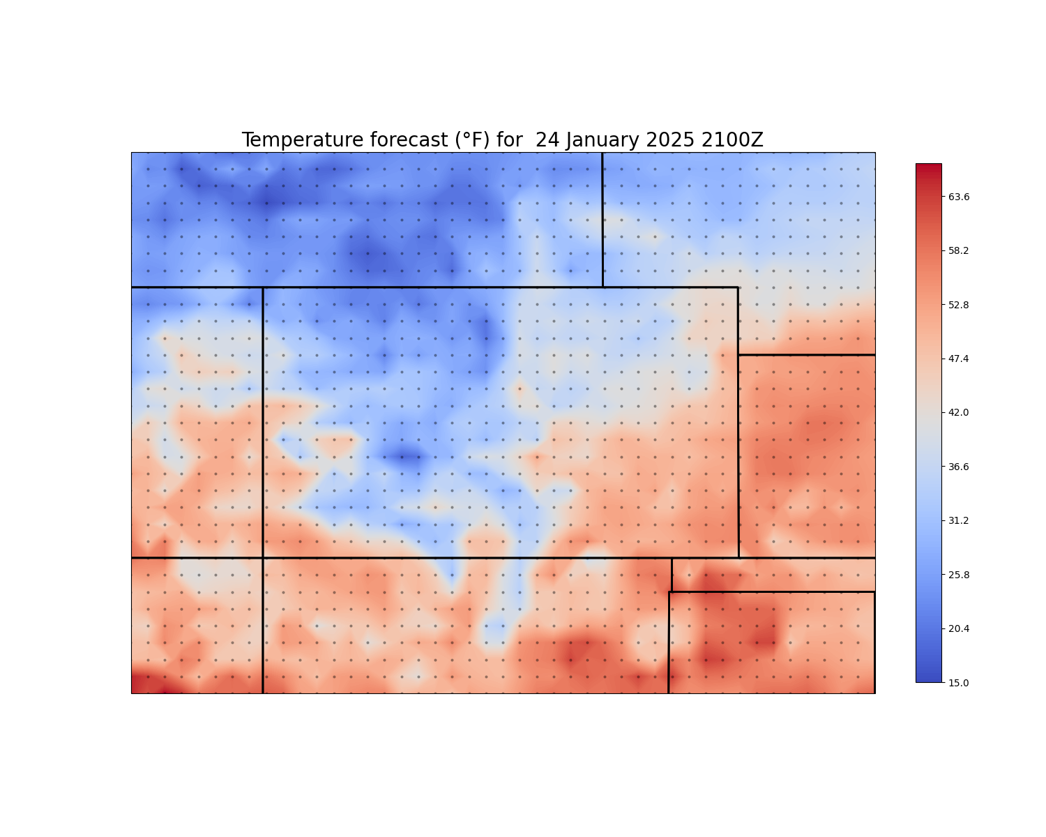
Now we can plot these up using matplotlib and cartopy.

# Create a new figure
fig = plt.figure(figsize=(15, 12))

# Add the map and set the extent
ax = plt.axes(projection=ccrs.PlateCarree())
ax.set_extent([-100., -111., 35, 43])

# Add state boundaries to plot
ax.add_feature(cfeature.STATES.with_scale('50m'), linewidth=2)

# Contour temperature at each lat/long
cf = ax.contourf(lon_2d, lat_2d, temp_vals, 200, transform=ccrs.PlateCarree(), zorder=0,
                 cmap='coolwarm')

# Plot a colorbar to show temperature and reduce the size of it
plt.colorbar(cf, ax=ax, fraction=0.032)

# Make a title with the time value
ax.set_title(u'Temperature forecast (\u00b0F) for {0:%d %B %Y %H:%MZ}'.format(time_val),
             fontsize=20)

# Plot markers for each lat/long to show grid points for 0.25 deg GFS
ax.plot(lon_2d.flatten(), lat_2d.flatten(), marker='o', color='black', markersize=2,
        alpha=0.3, transform=ccrs.Geodetic(), zorder=2, linestyle='none')

Total running time of the script: ( 0 minutes 6.179 seconds)