Forecast Model Vertical Sounding
Notebook Python-AWIPS Tutorial Notebook
Objectives
Use python-awips to connect to an edex server
Request data using the ModelSounding class in addition to using the normal DataAccess class
Create and compare vertical sounding from different AWIPS model data with isobaric levels
Use Shapely Point geometry to define a point
Convert between units when necessary
Table of Contents
1 Imports
The imports below are used throughout the notebook. Note the first import is coming directly from python-awips and allows us to connect to an EDEX server. The subsequent imports are for data manipulation and visualization.
from awips.dataaccess import DataAccessLayer, ModelSounding
import matplotlib.pyplot as plt
import numpy as np
from metpy.plots import SkewT, Hodograph
from metpy.units import units
from mpl_toolkits.axes_grid1.inset_locator import inset_axes
from math import sqrt
from shapely.geometry import Point
2 EDEX Connection
First we establish a connection to Unidata’s public EDEX server. This sets the proper server on the DataAccessLayer, which we will use numerous times throughout the notebook.
server = 'edex-cloud.unidata.ucar.edu'
DataAccessLayer.changeEDEXHost(server)
3 Define Useful Variables
The plotting in this notebook needs a model name, a location point (defined by latitude and longitude), and the most recent time range with the initial forecast run.
# Note the order is Lon,Lat and not Lat,Lon
point = Point(-104.67,39.87)
model="NAM40"

# Get latest forecast cycle run
timeReq = DataAccessLayer.newDataRequest("grid")
timeReq.setLocationNames(model)
cycles = DataAccessLayer.getAvailableTimes(timeReq, True)
times = DataAccessLayer.getAvailableTimes(timeReq)
fcstRun = DataAccessLayer.getForecastRun(cycles[-2], times)

timeRange = [fcstRun[0]]

print("Using " + model + " forecast time " + str(timeRange))
Using NAM40 forecast time [<DataTime instance: 2023-07-25 12:00:00 >]
4 Function: get_surface_data()
This function is used to get the initial forecast model data for surface height. This is done separately from the rest of the heights to determine the surface pressure. It uses the ModelSounding data object from python-awips to retrieve all the relevant information.
This function takes the model name, location, and time as attributes, and returns arrays for pressure, temperature, dewpoint, and the u and v wind components.
def get_surface_data(modelName, location, time):
    """ model name, location, and timeRange desire """

    # request data and sort response
    pressure,temp,dpt,ucomp,vcomp = [],[],[],[],[]
    use_parms = ['T','DpT','uW','vW','P']
    use_level = "0.0FHAG"

    sndObject = ModelSounding.getSounding(modelName, use_parms, [use_level], location, time)
    if len(sndObject) > 0:
        for time in sndObject._dataDict:
            pressure.append(float(sndObject._dataDict[time][use_level]['P']))
            temp.append(float(sndObject._dataDict[time][use_level]['T']))
            dpt.append(float(sndObject._dataDict[time][use_level]['DpT']))
            ucomp.append(float(sndObject._dataDict[time][use_level]['uW']))
            vcomp.append(float(sndObject._dataDict[time][use_level]['vW']))
        print("Found surface record at " + "%.1f" % pressure[0] + "MB")
    else:
        raise ValueError("sndObject returned empty for query ["
                        + ', '.join(str(x) for x in (modelName, use_parms, point, use_level)) +"]")

    # return information for plotting
    return pressure,temp,dpt,ucomp,vcomp
5 Function: get_levels_data()
This function is similar to get_surface_data(), except it gets data values for presure heights above the surface. It uses the ModelSounding data object from python-awips to retrieve all the relevant information.
It takes the model name, location, and time (similar to the other function), and also takes the instantiated pressure, temperature, dewpoint, and wind vector arrays.
It returns the fully populated pressure, temperature, dewpoint, u-component, v-component, and computed wind arrays.
def get_levels_data(modelName, location, time, pressure, temp, dpt, ucomp, vcomp):

    # Get isobaric levels with our requested parameters
    parms = ['T','DpT','uW','vW']
    levelReq = DataAccessLayer.newDataRequest("grid", envelope=point)
    levelReq.setLocationNames(model)
    levelReq.setParameters(*(parms))
    availableLevels = DataAccessLayer.getAvailableLevels(levelReq)

    # Clean levels list of unit string (MB, FHAG, etc.)
    levels = []
    for lvl in availableLevels:
        name=str(lvl)
        if 'MB' in name and '_' not in name:
            # If this level is above (less than in mb) our 0.0FHAG record
            if float(name.replace('MB','')) < pressure[0]:
                levels.append(lvl)

    # Get Sounding
    sndObject = ModelSounding.getSounding(modelName, parms, levels, location, time)

    if not len(sndObject) > 0:
        raise ValueError("sndObject returned empty for query ["
                        + ', '.join(str(x) for x in (model, parms, point, levels)) +"]")

    for time in sndObject._dataDict:
        for lvl in sndObject._dataDict[time].levels():
            for parm in sndObject._dataDict[time][lvl].parameters():
                if parm == "T":
                    temp.append(float(sndObject._dataDict[time][lvl][parm]))
                elif parm == "DpT":
                    dpt.append(float(sndObject._dataDict[time][lvl][parm]))
                elif parm == 'uW':
                    ucomp.append(float(sndObject._dataDict[time][lvl][parm]))
                elif parm == 'vW':
                    vcomp.append(float(sndObject._dataDict[time][lvl][parm]))
                else:
                    print("WHAT IS THIS")
                    print(sndObject._dataDict[time][lvl][parm])
            # Pressure is our requested level rather than a returned parameter
            pressure.append(float(lvl.replace('MB','')))

    # convert to numpy.array()
    pressure = np.array(pressure, dtype=float)
    temp = (np.array(temp, dtype=float) - 273.15) * units.degC
    dpt = (np.array(dpt, dtype=float) - 273.15) * units.degC
    ucomp = (np.array(ucomp, dtype=float) * units('m/s')).to('knots')
    vcomp = (np.array(vcomp, dtype=float) * units('m/s')).to('knots')
    wind = np.sqrt(ucomp**2 + vcomp**2)

    print("Using " + str(len(levels)) + " levels between " +
          str("%.1f" % max(pressure)) + " and " + str("%.1f" % min(pressure)) + "MB")
    return pressure,temp,dpt,ucomp,vcomp,wind
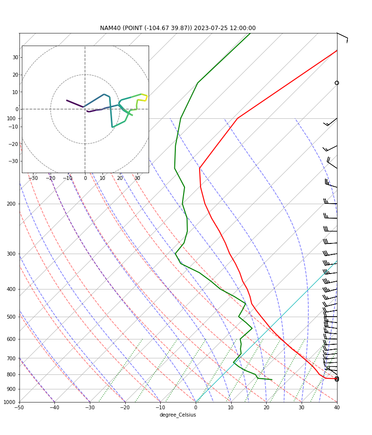
6 Function: plot_skewT()
Since we’re plotting many different models for comparison, all that code was used to create this function.
The function takes the model name, reference time, and the pressure, temperature, dewpoint, u-component, v-component, and wind arrays. It plots a skewT and hodograph using metpy.
def plot_skewT(modelName, pressure, temp, dpt, ucomp, vcomp, wind, refTime):
    plt.rcParams['figure.figsize'] = (12, 14)

    # Skew-T
    skew = SkewT(rotation=45)
    skew.plot(pressure, temp, 'r', linewidth=2)
    skew.plot(pressure, dpt, 'g', linewidth=2)
    skew.plot_barbs(pressure, ucomp, vcomp)
    skew.plot_dry_adiabats()
    skew.plot_moist_adiabats()
    skew.plot_mixing_lines(linestyle=':')

    skew.ax.set_ylim(1000, np.min(pressure))
    skew.ax.set_xlim(-50, 40)

    # Title
    plt.title(modelName + " (" + str(point) + ") " + str(refTime))

    # Hodograph
    ax_hod = inset_axes(skew.ax, '40%', '40%', loc=2)
    h = Hodograph(ax_hod, component_range=max(wind.magnitude))
    h.add_grid(increment=20)
    h.plot_colormapped(ucomp, vcomp, wind)

    # Dotted line at 0C isotherm
    l = skew.ax.axvline(0, color='c', linestyle='-', linewidth=1)

    plt.show()
7 Retrieve Necessary Plotting Data
First we get the initial data at surface level using the get_surface_data function, and then pass those initial data arrays onto the get_levels_data request to finish populating for additional heights needed for Skew-T plots. We want to keep track of the pressure, temeperature, dewpoint, u-component, v-component, and wind arrays so we store them in variables to use later on.
p,t,d,u,v = get_surface_data(model,point,timeRange)

p,t,d,u,v,w = get_levels_data(model,point,timeRange,p,t,d,u,v)
Found surface record at 833.2MB
Using 32 levels between 833.2 and 50.0MB
8 Skew-T/Log-P
Here we use our plot_skewT function to generate our skewT & hodograph charts for the data we retreived so far. This is where the pressure, temperature, dewpoint, and wind data is needed.
plot_skewT(model, p, t, d, u, v, w, timeRange[0])
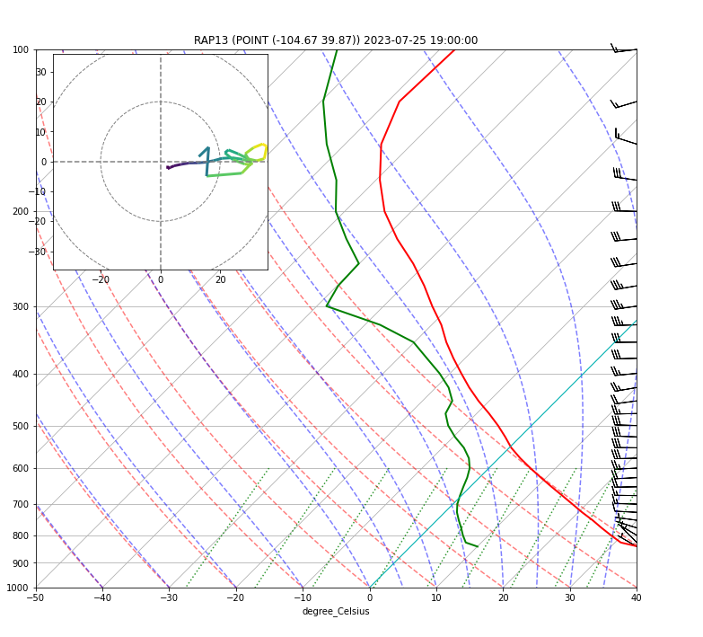
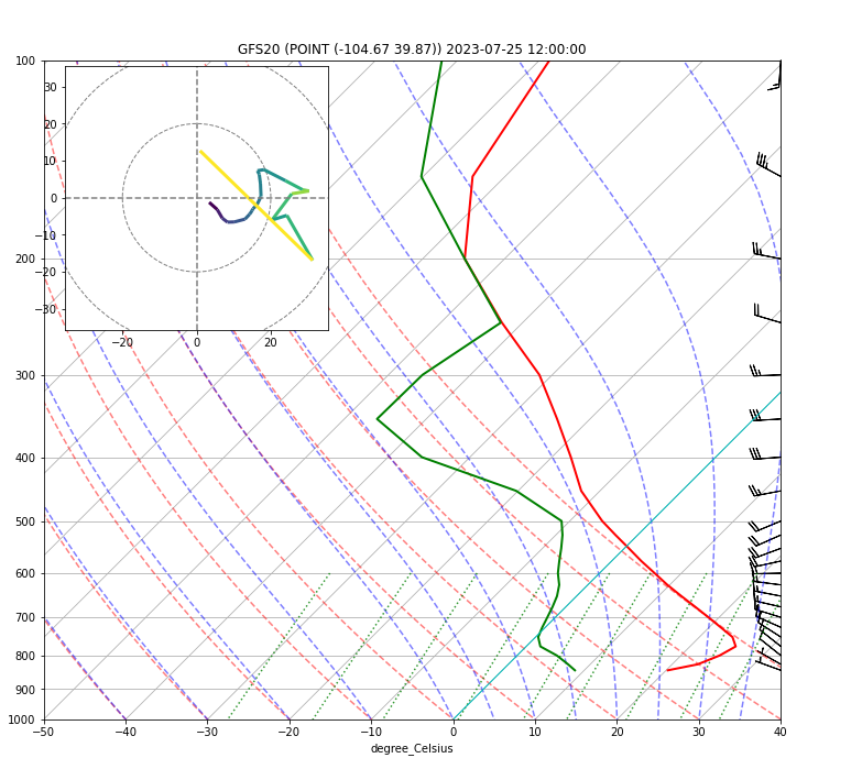
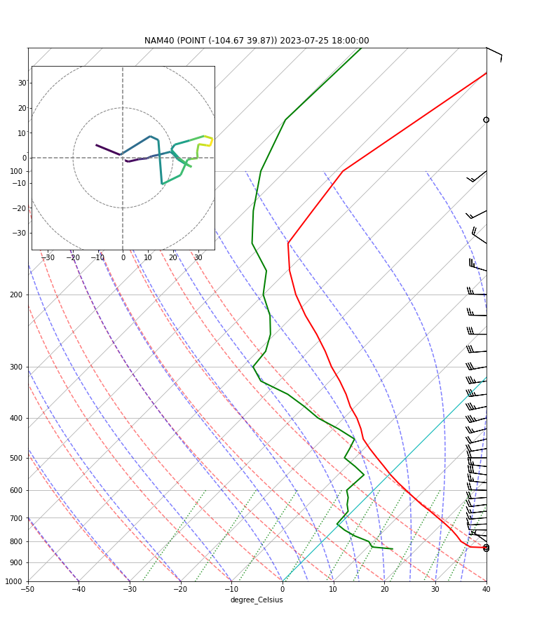
9 Model Sounding Comparison
Now that we know how to retreive and plot the data for one model, we can run a loop to retreive data for various models and plot them for comparison. In this example we’ll also plot RAP13 and GFS20 data to compare with NAM40.
This is also where our functions become so important, because we can easily recall all that logic and keep this for-loop fairly simple.
models = ["RAP13", "GFS20", "NAM40"]

for modelName in models:
    timeReq = DataAccessLayer.newDataRequest("grid")
    timeReq.setLocationNames(modelName)
    cycles = DataAccessLayer.getAvailableTimes(timeReq, True)
    times = DataAccessLayer.getAvailableTimes(timeReq)
    fr = DataAccessLayer.getForecastRun(cycles[-1], times)
    print("Using " + modelName + " forecast time " + str(fr[0]))
    tr = [fr[0]]

    p,t,d,u,v = get_surface_data(modelName,point,tr)
    p,t,d,u,v,w = get_levels_data(modelName,point,tr,p,t,d,u,v)

    # Skew-T
    plot_skewT(modelName,p,t,d,u,v,w,tr[0])
Using RAP13 forecast time 2023-07-25 19:00:00
Found surface record at 839.4MB
Using 32 levels between 839.4 and 100.0MB
Using GFS20 forecast time 2023-07-25 12:00:00
Found surface record at 842.5MB
Using 32 levels between 842.5 and 100.0MB
Using NAM40 forecast time 2023-07-25 18:00:00
Found surface record at 833.8MB
Using 32 levels between 833.8 and 50.0MB
10 See Also
10.2 Additional Documentation
python-awips:
matplotlib:
MetPy