Map Resources and Topography
Notebook Python-AWIPS Tutorial Notebook
Objectives
Use python-awips to connect to an edex server
Define data request object specifically for the maps database
Manipulate request object for various different map resources
Plot map resources in combination with one another for geographical context
Table of Contents
1 Imports
The imports below are used throughout the notebook. Note the first import is coming directly from python-awips and allows us to connect to an EDEX server. The subsequent imports are for data manipulation and visualization.
from awips.dataaccess import DataAccessLayer
import matplotlib.pyplot as plt
import cartopy.crs as ccrs
import numpy.ma as ma
from cartopy.mpl.gridliner import LONGITUDE_FORMATTER, LATITUDE_FORMATTER
from cartopy.feature import ShapelyFeature,NaturalEarthFeature
from shapely.ops import unary_union
2 Connect to EDEX
First we establish a connection to Unidata’s public EDEX server. With that connection made, we can create a new data request object and set the data type to maps.
# Server, Data Request Type, and Database Table
DataAccessLayer.changeEDEXHost("edex-cloud.unidata.ucar.edu")
request = DataAccessLayer.newDataRequest('maps')
3 Function: make_map()
In many of our notebooks we end up plotting map images, and this logic below is the same from those other notebooks. Typically, functions are defined when they are called multiple times throughout a notebook. In this case, we only use it in one code block cell, but because it is a common function from several of our notebooks, it’s nice to keep the logic neatly defined for consistency.
# Standard map plot
def make_map(bbox, projection=ccrs.PlateCarree()):
    fig, ax = plt.subplots(figsize=(12,12),
            subplot_kw=dict(projection=projection))
    ax.set_extent(bbox)
    ax.coastlines(resolution='50m')
    gl = ax.gridlines(draw_labels=True)
    gl.top_labels = gl.right_labels = False
    gl.xformatter = LONGITUDE_FORMATTER
    gl.yformatter = LATITUDE_FORMATTER
    return fig, ax
4 Create Initial Map From CWA
The python-awips package provides access to the entire AWIPS Maps Database for use in Python GIS applications. Map objects are returned as Shapely geometries and can be easily plotted by many Python packages.
Each map database table has a geometry field called
the_geom, which can be used to spatially select map resources for any column of type geometry.
Tip: Note the geometry definition of
the_geomfor each data type, which can be Point, MultiPolygon, or MultiLineString.
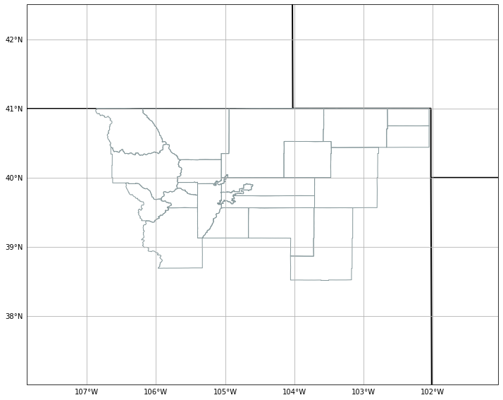
Here we’ll be using Boulder (BOU) as our example for plotting the County Warning Area (CWA). We’ll query our EDEX server to get all counties in the CWA for BOU, and then plot those counties along withe the state boundaries and lines of longitude and latitude. In order to get this information from EDEX, we’ll need to set several characteristics on our data request object. We will use request.setParameters() to refine our query to EDEX.
# Specify the necessary identifiers for requesting the Boulder CWA
request.addIdentifier('table', 'mapdata.county')
# Define a WFO ID for location
# tie this ID to the mapdata.county column "cwa" for filtering
request.setLocationNames('BOU')
request.addIdentifier('cwa', 'BOU')
# enable location filtering (inLocation)
# locationField is tied to the above cwa definition (BOU)
request.addIdentifier('geomField', 'the_geom')
request.addIdentifier('inLocation', 'true')
request.addIdentifier('locationField', 'cwa')

# Get response and create dict of county geometries
response = DataAccessLayer.getGeometryData(request)
counties = []
for ob in response:
    counties.append(ob.getGeometry())
print("Using " + str(len(counties)) + " county MultiPolygons")


# All WFO counties merged to a single Polygon
merged_counties = unary_union(counties)
envelope = merged_counties.buffer(2)
boundaries=[merged_counties]

# Get bounds of this merged Polygon to use as buffered map extent
bounds = merged_counties.bounds
bbox=[bounds[0]-1,bounds[2]+1,bounds[1]-1.5,bounds[3]+1.5]

# Create the map we'll use for the rest of this notebook based on the
# boundaries of the CWA
fig, ax = make_map(bbox=bbox)

# Plot political/state boundaries handled by Cartopy
political_boundaries = NaturalEarthFeature(category='cultural',
                               name='admin_0_boundary_lines_land',
                               scale='50m', facecolor='none')
states = NaturalEarthFeature(category='cultural',
                               name='admin_1_states_provinces_lines',
                               scale='50m', facecolor='none')
ax.add_feature(political_boundaries, linestyle='-', edgecolor='black')
ax.add_feature(states, linestyle='-', edgecolor='black',linewidth=2)

# Plot CWA counties
shape_feature = ShapelyFeature(counties,ccrs.PlateCarree(),
                    facecolor='none', linestyle="-",edgecolor='#86989B')
ax.add_feature(shape_feature)
Using 22 county MultiPolygons
<cartopy.mpl.feature_artist.FeatureArtist at 0x11568f6d0>
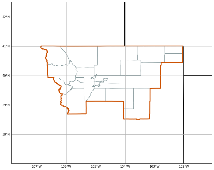
5 Draw Merged CWA
In the previous section we created a merged polygon with the applicable counties. Here, we draw this new shape on top of our existing map in a burnt orange color.
# Plot CWA envelope
shape_feature = ShapelyFeature(boundaries,ccrs.PlateCarree(),
                    facecolor='none', linestyle="-",linewidth=3.,edgecolor='#cc5000')
ax.add_feature(shape_feature)

fig
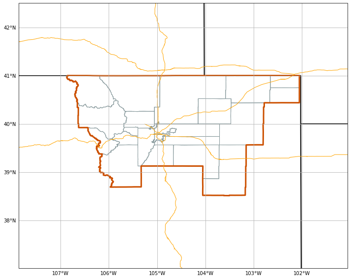
6 Draw Interstates using Boundary Filter
Now, we’ll use the previously-defined envelope=merged_counties.buffer(2) in a newDataRequest() to request interstate geometries which fall inside the buffered boundary.
# Define the request for the interstate query
request = DataAccessLayer.newDataRequest('maps', envelope=envelope)
request.addIdentifier('table', 'mapdata.interstate')
request.addIdentifier('geomField', 'the_geom')
interstates = DataAccessLayer.getGeometryData(request)
print("Using " + str(len(interstates)) + " interstate MultiLineStrings")

# Plot interstates
for ob in interstates:
    shape_feature = ShapelyFeature(ob.getGeometry(),ccrs.PlateCarree(),
                        facecolor='none', linestyle="-",edgecolor='orange')
    ax.add_feature(shape_feature)
fig
Using 225 interstate MultiLineStrings
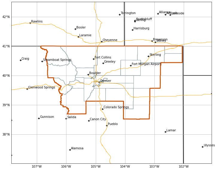
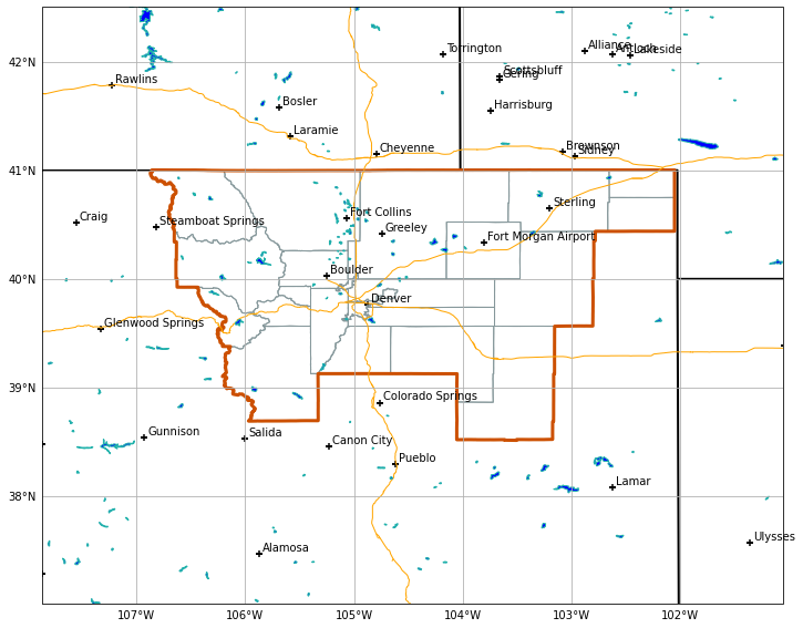
7 Draw Nearby Cities
Request the city table based using the envelope attribute and filter by population and progressive disclosure level.
Warning: The
prog_discfield is not entirely understood and values appear to change significantly depending on WFO site.
# Define the request for the city query
request = DataAccessLayer.newDataRequest('maps', envelope=envelope)
request.addIdentifier('table', 'mapdata.city')
request.addIdentifier('geomField', 'the_geom')
request.setParameters('name','population','prog_disc')
cities = DataAccessLayer.getGeometryData(request)
print("Queried " + str(len(cities)) + " total cities")

# Set aside two arrays - one for the geometry of the cities and one for their names
citylist = []
cityname = []
# For BOU, progressive disclosure values above 50 and pop above 5000 looks good
for ob in cities:
    if ob.getString("population") != 'None':
        if ob.getNumber("prog_disc") > 50 and int(ob.getString("population")) > 5000:
            citylist.append(ob.getGeometry())
            cityname.append(ob.getString("name"))
print("Plotting " + str(len(cityname)) + " cities")

# Plot city markers
ax.scatter([point.x for point in citylist],
       [point.y for point in citylist],
       transform=ccrs.PlateCarree(),marker="+",facecolor='black')
# Plot city names
for i, txt in enumerate(cityname):
    ax.annotate(txt, (citylist[i].x,citylist[i].y),
                xytext=(3,3), textcoords="offset points")

fig
Queried 1205 total cities
Plotting 58 cities
8 Draw Nearby Lakes
Again, use the envelope attribute to define a new data requst for the nearby lakes.
# Define request for lakes
request = DataAccessLayer.newDataRequest('maps', envelope=envelope)
request.addIdentifier('table', 'mapdata.lake')
request.addIdentifier('geomField', 'the_geom')

# Get lake geometries
response = DataAccessLayer.getGeometryData(request)
print("Using " + str(len(response)) + " lake MultiPolygons")

# Plot lakes
shape_feature = ShapelyFeature([lake.getGeometry() for lake in response],ccrs.PlateCarree(),
                    facecolor='blue', linestyle="-",edgecolor='#20B2AA')
ax.add_feature(shape_feature)
fig
Using 208 lake MultiPolygons
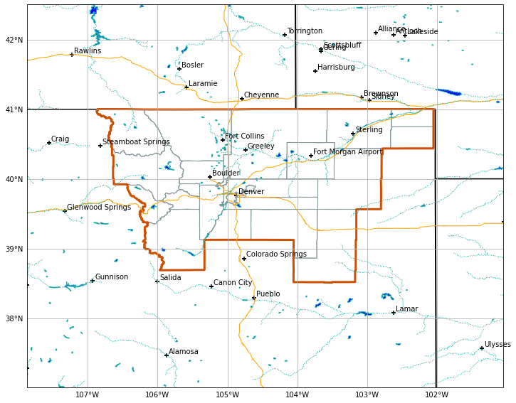
9 Draw Major Rivers
# Define request for rivers
request = DataAccessLayer.newDataRequest('maps', envelope=envelope)
request.addIdentifier('table', 'mapdata.majorrivers')
request.addIdentifier('geomField', 'the_geom')
rivers = DataAccessLayer.getGeometryData(request)
print("Using " + str(len(rivers)) + " river MultiLineStrings")

# Plot rivers
shape_feature = ShapelyFeature([river.getGeometry() for river in rivers],ccrs.PlateCarree(),
                    facecolor='none', linestyle=":",edgecolor='#20B2AA')
ax.add_feature(shape_feature)
fig
Using 1400 river MultiLineStrings
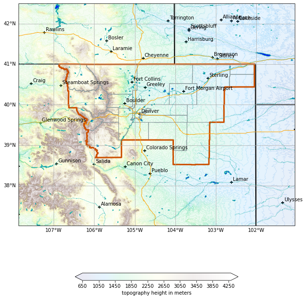
10 Draw Topography
Spatial envelopes are required for topo requests, which can become slow to download and render for large (CONUS) maps.
# Define topography request
request = DataAccessLayer.newDataRequest("topo", envelope=envelope)
request.addIdentifier("group", "/")
request.addIdentifier("dataset", "full")
gridData = DataAccessLayer.getGridData(request)
print(gridData)
print("Number of grid records: " + str(len(gridData)))
print("Sample grid data shape:\n" + str(gridData[0].getRawData().shape) + "\n")
print("Sample grid data:\n" + str(gridData[0].getRawData()) + "\n")
[<awips.dataaccess.PyGridData.PyGridData object at 0x115a20370>]
Number of grid records: 1
Sample grid data shape:
(778, 1058)

Sample grid data:
[[1694. 1693. 1688. ...  757.  761.  762.]
 [1701. 1701. 1701. ...  758.  760.  762.]
 [1703. 1703. 1703. ...  760.  761.  762.]
 ...
 [1767. 1741. 1706. ...  769.  762.  768.]
 [1767. 1746. 1716. ...  775.  765.  761.]
 [1781. 1753. 1730. ...  766.  762.  759.]]
grid=gridData[0]
topo=ma.masked_invalid(grid.getRawData())
lons, lats = grid.getLatLonCoords()
print(topo.min()) # minimum elevation in our domain (meters)
print(topo.max()) # maximum elevation in our domain (meters)

# Plot topography
cs = ax.contourf(lons, lats, topo, 80, cmap=plt.get_cmap('terrain'),alpha=0.1, extend='both')
cbar = fig.colorbar(cs, shrink=0.5, orientation='horizontal')
cbar.set_label("topography height in meters")

fig
623.0
4328.0
11 See Also
11.1 Additional Documentation
This notebook requires: python-awips, numpy, matplotplib, cartopy, shapely
Use datatype maps and addIdentifier(‘table’, <postgres maps schema>) to define the map table: DataAccessLayer.changeEDEXHost(“edex-cloud.unidata.ucar.edu”) request = DataAccessLayer.newDataRequest(‘maps’) request.addIdentifier(‘table’, ‘mapdata.county’)
Use request.setLocationNames() and request.addIdentifier() to spatially filter a map resource. In the example below, WFO ID BOU (Boulder, Colorado) is used to query counties within the BOU county watch area (CWA)
request.addIdentifier('geomField', 'the_geom')
request.addIdentifier('inLocation', 'true')
request.addIdentifier('locationField', 'cwa')
request.setLocationNames('BOU')
request.addIdentifier('cwa', 'BOU')
See the Maps Database Reference Page for available database tables, column names, and types.