Getting Started with MetPy
Welcome to MetPy! We’re glad you’re here and we hope that you find this Python library to be useful for your needs. In order to help get you started with MetPy, we’ve put together this guide to introduce you to the basic syntax and functionality of this library. If you’re new to Python, please visit the Unidata Python Training site for in-depth discussion and examples of the Scientific Python ecosystem.
For installation instructions, please see our Install Guide.
Units
For the in-depth explanation of units, associated syntax, and unique features, please see our Units Tutorial page. What follows in this section is a short summary of how MetPy uses units.
One of the most significant differences in syntax for MetPy, compared to other Python libraries, is the frequent requirement of units to be attached to arrays before being passed to MetPy functions. There are very few exceptions to this, and you’ll usually be safer to always use units whenever applicable to make sure that your analyses are done correctly. Once you get used to the units syntax, it becomes very handy, as you never have to worry about unit conversion for any calculation. MetPy does it for you!
To demonstrate the units syntax briefly here, we can do this:
import numpy as np
from metpy.units import units

distance = np.arange(1, 5) * units.meters
Another way to attach units is do create the array directly with the pint.Quantity
object:
time = units.Quantity(np.arange(2, 10, 2), 'sec')
Unit-aware calculations can then be done with these variables:
print(distance / time)
[ 0.5 0.5 0.5 0.5] meter / second
In addition to the Units Tutorial page, checkout the MetPy Monday blog on units or watch our MetPy Monday video on temperature units.
Functionality
MetPy aims to have three primary purposes: read and write meteorological data (I/O), calculate meteorological quantities with well-documented equations, and create publication-quality plots of meteorological data. The three subsections that follow will demonstrate just some of this functionality. For full reference to all of MetPy’s API, please see our Reference Guide.
Input/Output
MetPy has built in support for reading GINI satellite and NEXRAD radar files. If you have one of these files, opening it with MetPy is as easy as:
from metpy.io import Level2File, Level3File, GiniFile

f = GiniFile(example_filename.gini)
f = Level2File(example_filename.gz)
f = Level3File(example_filename.gz)
From there, you can pull out the variables you want to analyze and plot. For more information, see the GINI, NEXRAD Level 2, and NEXRAD Level 3 examples. MetPy Monday videos #29 and #30 also show how to plot radar files with MetPy.
The other exciting feature is MetPy’s Xarray accessor. Xarray is a Python package that makes working with multi-dimensional labeled data (i.e. netCDF files) easy. For a thorough look at Xarray’s capabilities, see this MetPy Monday video. With MetPy’s accessor to this package, we can quickly pull out common dimensions, parse Climate and Forecasting (CF) metadata, and handle projection information. While the Xarray with MetPy is the best place to see the full utility of the MetPy Xarray accessor, let’s demonstrate some of the functionality here:
import xarray as xr
import metpy
from metpy.cbook import get_test_data

ds = xr.open_dataset(get_test_data('narr_example.nc', as_file_obj = False))
ds = ds.metpy.parse_cf()

# Grab lat/lon values from file as unit arrays
lats = ds.lat.metpy.unit_array
lons = ds.lon.metpy.unit_array

# Get the valid time
vtime = ds.Temperature_isobaric.metpy.time[0]

# Get the 700-hPa heights without manually identifying the vertical coordinate
hght_700 = ds.Geopotential_height_isobaric.metpy.sel(vertical=700 * units.hPa,
                                                 time=vtime)
From here, you could make a map of the 700-hPa geopotential heights. We’ll discuss how to do that in the Plotting section.
Calculations
Meteorology and atmospheric science are fully-dependent on complex equations and formulas. Rather than figuring out how to write them efficiently in Python yourself, MetPy provides support for many of the common equations within the field. For the full list, please see the Calculations reference guide. If you don’t see the equation you’re looking for, consider submitting a feature request to MetPy here.
To demonstrate some of the calculations MetPy can do, let’s show a simple example:
import numpy as np
from metpy.units import units
import metpy.calc as mpcalc

temperature = [20] * units.degC
rel_humidity  = [50] * units.percent
print(mpcalc.dewpoint_from_relative_humidity(temperature, rel_humidity))
array([9.27008599]) <Unit('degC')>
speed = np.array([5, 10, 15, 20]) * units.knots
direction = np.array([0, 90, 180, 270]) * units.degrees
u, v = mpcalc.wind_components(speed, direction)
print(u, v)
[0 -10 0 20] knot
[-5 0 15 0] knot
As discussed above, if you don’t provide units to these functions, they will frequently fail with the following error:
ValueError: calculation given arguments with incorrect units: variable requires
"[type of unit]" but given "none". Any variable x can be assigned a unit as follows:
from metpy.units import units
x = x * units.meter / units.second
If you see this error in your code, just attach the appropriate units and you’ll be good to go!
Plotting
MetPy contains two special types of meteorological plots, the Skew-T Log-P and Station plots, that more general Python plotting packages don’t support as readily. Additionally, with the goal to replace GEMPAK, MetPy’s declarative plotting interface is being actively developed, which will make plotting a simple task with straight-forward syntax, similar to GEMPAK.
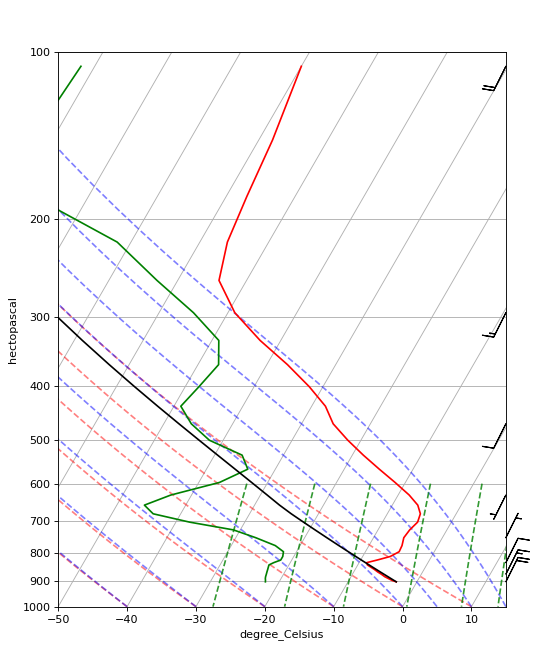
Skew-T
The Skew-T Log-P diagram is the canonical thermodynamic diagram within meteorology. Using
matplotlib, MetPy is able to readily create a Skew-T for you:
import matplotlib.pyplot as plt
import numpy as np
import metpy.calc as mpcalc
from metpy.plots import SkewT
from metpy.units import units

fig = plt.figure(figsize=(9, 9))
skew = SkewT(fig)

# Create arrays of pressure, temperature, dewpoint, and wind components
p = [902, 897, 893, 889, 883, 874, 866, 857, 849, 841, 833, 824, 812, 796, 776, 751,
     727, 704, 680, 656, 629, 597, 565, 533, 501, 468, 435, 401, 366, 331, 295, 258,
     220, 182, 144, 106] * units.hPa
t = [-3, -3.7, -4.1, -4.5, -5.1, -5.8, -6.5, -7.2, -7.9, -8.6, -8.9, -7.6, -6, -5.1,
     -5.2, -5.6, -5.4, -4.9, -5.2, -6.3, -8.4, -11.5, -14.9, -18.4, -21.9, -25.4,
     -28, -32, -37, -43, -49, -54, -56, -57, -58, -60] * units.degC
td = [-22, -22.1, -22.2, -22.3, -22.4, -22.5, -22.6, -22.7, -22.8, -22.9, -22.4,
      -21.6, -21.6, -21.9, -23.6, -27.1, -31, -38, -44, -46, -43, -37, -34, -36,
      -42, -46, -49, -48, -47, -49, -55, -63, -72, -88, -93, -92] * units.degC
# Calculate parcel profile
prof = mpcalc.parcel_profile(p, t[0], td[0]).to('degC')
u = np.linspace(-10, 10, len(p)) * units.knots
v = np.linspace(-20, 20, len(p)) * units.knots

skew.plot(p, t, 'r')
skew.plot(p, td, 'g')
skew.plot(p, prof, 'k')  # Plot parcel profile
skew.plot_barbs(p[::5], u[::5], v[::5])

skew.ax.set_xlim(-50, 15)
skew.ax.set_ylim(1000, 100)

# Add the relevant special lines
skew.plot_dry_adiabats()
skew.plot_moist_adiabats()
skew.plot_mixing_lines()

plt.show()
For some MetPy Monday videos on Skew-Ts, please watch #16, #18, and #19. Hodographs can also be created and plotted with a Skew-T (see MetPy Monday video #38). For more examples on how to do create Skew-Ts and Hodographs, please visit check out the Simple Sounding, Advanced Sounding, and Hodograph Inset.
Station Plots
Station plots display surface or upper-air station data in a concise manner. The creation of
these plots is made straightforward with MetPy. MetPy supplies the ability to create each
station plot and place the points on the map. The creation of 2-D cartographic maps, commonly
used in meteorology for observational and model visualization, relies upon the CartoPy
library. This package handles projections and transforms to make sure your data is plotted in
the correct location.
For examples on how to make a station plot, please see the Station Plot and Station Plot Layout examples.
Gridded Data
While MetPy doesn’t provide many new tools for 2-D gridded data maps, we do provide lots of examples illustrating how to use MetPy for data analysis and CartoPy for visualization. Those examples can be found in the MetPy Gallery and at the Unidata Python Training site.
One unique tool in MetPy for gridded data is cross-section analysis. A detailed example of how to create a cross section with your gridded data is available here.
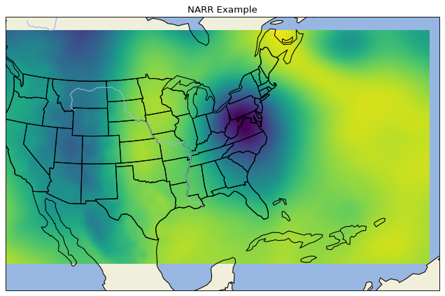
Declarative Plotting
The declarative plotting interface, which is still under active development, aims to replicate the simple plotting declarations in GEMPAK to make map creation straightforward, especially for those less familiar with Python, CartoPy, and matplotlib. To demonstrate the ease of creating a plot with this interface, let’s make a color-filled plot of temperature using NARR data.
import xarray as xr
from metpy.cbook import get_test_data
from metpy.plots import ImagePlot, MapPanel, PanelContainer
from metpy.units import units

# Use sample NARR data for plotting
narr = xr.open_dataset(get_test_data('narr_example.nc', as_file_obj=False))

img = ImagePlot()
img.data = narr
img.field = 'Geopotential_height'
img.level = 850 * units.hPa

panel = MapPanel()
panel.area = 'us'
panel.layers = ['coastline', 'borders', 'states', 'rivers', 'ocean', 'land']
panel.title = 'NARR Example'
panel.plots = [img]

pc = PanelContainer()
pc.size = (10, 8)
pc.panels = [panel]
pc.show()
Other plot types are available, including contouring to create overlay maps. For an example of this, check out the Combined Plotting example. MetPy Monday videos #69, #70, and #71 also demonstrate the declarative plotting interface.
Other Python Resources
While MetPy does a lot of things, it doesn’t do everything. Here are some other good resources to use as you start using MetPy and Python for meteorology and atmospheric science:
Learning Resources
Useful Python Packages
Siphon: remote access of meteorological data, including simple web services and and via THREDDS Data Servers
netCDF4-python is the officially blessed Python API for netCDF
Xarray: reading/writing labeled N-dimensional arrays
Pandas: reading/writing tabular data
NumPy: numerical computations
Matplotlib: creation of publication-quality figures
CartoPy: publication-quality cartographic maps
SatPy: read and visualize satellite data
PyART: read and visualize radar data
Support
Get stuck trying to use MetPy with your data? Unidata’s Python team is here to help! See our support page for more information.