SkewT¶

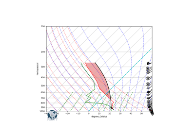
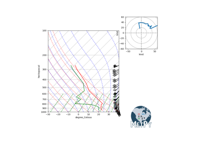
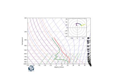
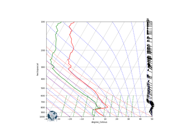
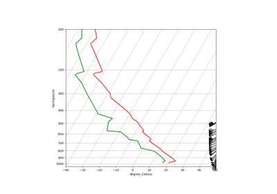
class metpy.plots.SkewT(fig=None, rotation=30, subplot=None, rect=None, aspect=80.5)[source]¶

Make Skew-T log-P plots of data.

This class simplifies the process of creating Skew-T log-P plots in using matplotlib. It handles requesting the appropriate skewed projection, and provides simplified wrappers to make it easy to plot data, add wind barbs, and add other lines to the plots (e.g. dry adiabats)

ax¶

The underlying Axes instance, which can be used for calling additional plot functions (e.g. axvline)

Type: matplotlib.axes.Axes

Create SkewT - logP plots.

Parameters

fig (matplotlib.figure.Figure, optional) – Source figure to use for plotting. If none is given, a new matplotlib.figure.Figure instance will be created.
rotation (float or int, optional) – Controls the rotation of temperature relative to horizontal. Given in degrees counterclockwise from x-axis. Defaults to 30 degrees.
subplot (tuple[int, int, int] or matplotlib.gridspec.SubplotSpec instance, optional) – Controls the size/position of the created subplot. This allows creating the skewT as part of a collection of subplots. If subplot is a tuple, it should conform to the specification used for matplotlib.figure.Figure.add_subplot(). The matplotlib.gridspec.SubplotSpec can be created by using matplotlib.gridspec.GridSpec.
rect (tuple[float, float, float, float], optional) – Rectangle (left, bottom, width, height) in which to place the axes. This allows the user to place the axes at an arbitrary point on the figure.
aspect (float, int, or 'auto', optional) – Aspect ratio (i.e. ratio of y-scale to x-scale) to maintain in the plot. Defaults to 80.5. Passing the string 'auto' tells matplotlib to handle the aspect ratio automatically (this is not recommended for SkewT).

Methods Summary

`__init__`([fig, rotation, subplot, rect, aspect])	Create SkewT - logP plots.
`plot`(pressure, t, args, *kwargs)	Plot data.
`plot_barbs`(pressure, u, v[, c, xloc, …])	Plot wind barbs.
`plot_dry_adiabats`([t0, pressure])	Plot dry adiabats.
`plot_mixing_lines`([mixing_ratio, pressure])	Plot lines of constant mixing ratio.
`plot_moist_adiabats`([t0, pressure])	Plot moist adiabats.
`shade_area`(y, x1[, x2, which])	Shade area between two curves.
`shade_cape`(pressure, t, t_parcel, **kwargs)	Shade areas of Convective Available Potential Energy (CAPE).
`shade_cin`(pressure, t, t_parcel[, dewpoint])	Shade areas of Convective INhibition (CIN).

Methods Documentation

__init__(fig=None, rotation=30, subplot=None, rect=None, aspect=80.5)[source]¶

Create SkewT - logP plots.

Parameters

fig (matplotlib.figure.Figure, optional) – Source figure to use for plotting. If none is given, a new matplotlib.figure.Figure instance will be created.
rotation (float or int, optional) – Controls the rotation of temperature relative to horizontal. Given in degrees counterclockwise from x-axis. Defaults to 30 degrees.
subplot (tuple[int, int, int] or matplotlib.gridspec.SubplotSpec instance, optional) – Controls the size/position of the created subplot. This allows creating the skewT as part of a collection of subplots. If subplot is a tuple, it should conform to the specification used for matplotlib.figure.Figure.add_subplot(). The matplotlib.gridspec.SubplotSpec can be created by using matplotlib.gridspec.GridSpec.
rect (tuple[float, float, float, float], optional) – Rectangle (left, bottom, width, height) in which to place the axes. This allows the user to place the axes at an arbitrary point on the figure.
aspect (float, int, or 'auto', optional) – Aspect ratio (i.e. ratio of y-scale to x-scale) to maintain in the plot. Defaults to 80.5. Passing the string 'auto' tells matplotlib to handle the aspect ratio automatically (this is not recommended for SkewT).

plot(pressure, t, *args, **kwargs)[source]¶

Plot data.

Simple wrapper around plot so that pressure is the first (independent) input. This is essentially a wrapper around plot.

Parameters

pressure (array_like) – pressure values
t (array_like) – temperature values, can also be used for things like dew point
args – Other positional arguments to pass to plot()
kwargs – Other keyword arguments to pass to plot()

Returns

list[matplotlib.lines.Line2D] – lines plotted

See also

matplotlib.pyplot.plot()

plot_barbs(pressure, u, v, c=None, xloc=1.0, x_clip_radius=0.1, y_clip_radius=0.08, **kwargs)[source]¶

Plot wind barbs.

Adds wind barbs to the skew-T plot. This is a wrapper around the barbs command that adds to appropriate transform to place the barbs in a vertical line, located as a function of pressure.

Parameters

pressure (array_like) – pressure values
u (array_like) – U (East-West) component of wind
v (array_like) – V (North-South) component of wind
c – An optional array used to map colors to the barbs
xloc (float, optional) – Position for the barbs, in normalized axes coordinates, where 0.0 denotes far left and 1.0 denotes far right. Defaults to far right.
x_clip_radius (float, optional) – Space, in normalized axes coordinates, to leave before clipping wind barbs in the x-direction. Defaults to 0.1.
y_clip_radius (float, optional) – Space, in normalized axes coordinates, to leave above/below plot before clipping wind barbs in the y-direction. Defaults to 0.08.
plot_units (pint.unit) – Units to plot in (performing conversion if necessary). Defaults to given units.
kwargs – Other keyword arguments to pass to barbs()

Returns

matplotlib.quiver.Barbs – instance created

See also

matplotlib.pyplot.barbs()

plot_dry_adiabats(t0=None, pressure=None, **kwargs)[source]¶

Plot dry adiabats.

Adds dry adiabats (lines of constant potential temperature) to the plot. The default style of these lines is dashed red lines with an alpha value of 0.5. These can be overridden using keyword arguments.

Parameters

t0 (array_like, optional) – Starting temperature values in Kelvin. If none are given, they will be generated using the current temperature range at the bottom of the plot.
pressure (array_like, optional) – Pressure values to be included in the dry adiabats. If not specified, they will be linearly distributed across the current plotted pressure range.
kwargs – Other keyword arguments to pass to matplotlib.collections.LineCollection

Returns

matplotlib.collections.LineCollection – instance created

plot_mixing_lines(mixing_ratio=None, pressure=None, **kwargs)[source]¶

Plot lines of constant mixing ratio.

Adds lines of constant mixing ratio (isohumes) to the plot. The default style of these lines is dashed green lines with an alpha value of 0.8. These can be overridden using keyword arguments.

Parameters

mixing_ratio (array_like, optional) – Unitless mixing ratio values to plot. If none are given, default values are used.
pressure (array_like, optional) – Pressure values to be included in the isohumes. If not specified, they will be linearly distributed across the current plotted pressure range up to 600 mb.
kwargs – Other keyword arguments to pass to matplotlib.collections.LineCollection

Returns

matplotlib.collections.LineCollection – instance created

See also

matplotlib.collections.LineCollection

plot_moist_adiabats(t0=None, pressure=None, **kwargs)[source]¶

Plot moist adiabats.

Adds saturated pseudo-adiabats (lines of constant equivalent potential temperature) to the plot. The default style of these lines is dashed blue lines with an alpha value of 0.5. These can be overridden using keyword arguments.

Parameters

t0 (array_like, optional) – Starting temperature values in Kelvin. If none are given, they will be generated using the current temperature range at the bottom of the plot.
pressure (array_like, optional) – Pressure values to be included in the moist adiabats. If not specified, they will be linearly distributed across the current plotted pressure range.
kwargs – Other keyword arguments to pass to matplotlib.collections.LineCollection

Returns

matplotlib.collections.LineCollection – instance created

shade_area(y, x1, x2=0, which='both', **kwargs)[source]¶

Shade area between two curves.

Shades areas between curves. Area can be where one is greater or less than the other or all areas shaded.

Parameters

y (array_like) – 1-dimensional array of numeric y-values
x1 (array_like) – 1-dimensional array of numeric x-values
x2 (array_like) – 1-dimensional array of numeric x-values
which (string) – Specifies if positive, negative, or both areas are being shaded. Will be overridden by where.
kwargs – Other keyword arguments to pass to matplotlib.collections.PolyCollection

Returns

matplotlib.collections.PolyCollection

See also

matplotlib.collections.PolyCollection, matplotlib.axes.Axes.fill_betweenx()

shade_cape(pressure, t, t_parcel, **kwargs)[source]¶

Shade areas of Convective Available Potential Energy (CAPE).

Shades areas where the parcel is warmer than the environment (areas of positive buoyancy.

Parameters

pressure (array_like) – Pressure values
t (array_like) – Temperature values
dewpoint (array_like) – Dewpoint values
t_parcel (array_like) – Parcel path temperature values
limit_shading (bool) – Eliminate shading below the LCL or above the EL, default is True
kwargs – Other keyword arguments to pass to matplotlib.collections.PolyCollection

Returns

matplotlib.collections.PolyCollection

See also

matplotlib.collections.PolyCollection, matplotlib.axes.Axes.fill_betweenx()

shade_cin(pressure, t, t_parcel, dewpoint=None, **kwargs)[source]¶

Shade areas of Convective INhibition (CIN).

Shades areas where the parcel is cooler than the environment (areas of negative buoyancy). If dewpoint is passed in, negative area below the lifting condensation level or above the equilibrium level is not shaded.

Parameters

pressure (array_like) – Pressure values
t (array_like) – Temperature values
t_parcel (array_like) – Parcel path temperature values
dewpoint (array_like) – Dew point values, optional
kwargs – Other keyword arguments to pass to matplotlib.collections.PolyCollection

Returns