Skew-T Layout

Notebook

import numpy as np
import matplotlib.pyplot as plt
import matplotlib.gridspec as gridspec

from metpy.cbook import get_test_data
from metpy.calc import get_wind_components
from metpy.plots import SkewT, Hodograph
from metpy.units import units

%matplotlib inline

# Parse the data
p, T, Td, direc, spd = np.loadtxt(get_test_data('may3_sounding.txt'),
        usecols=(0, 2, 3, 6, 7), skiprows=4, unpack=True)

# Add units to the data arrays
p = p * units.mbar
T = T * units.degC
Td = Td * units.degC
spd = spd * units.knot
direc = direc * units.deg

# Convert wind speed and direction to components
u, v = get_wind_components(spd, direc)

# Create a new figure. The dimensions here give a good aspect ratio
fig = plt.figure(figsize=(9, 9))

# Grid for plots
gs = gridspec.GridSpec(3, 3)
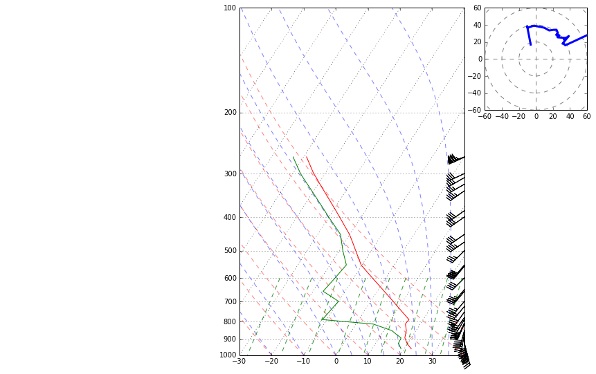
skew = SkewT(fig, rotation=45, subplot=gs[:, :2])

# Plot the data using normal plotting functions, in this case using
# log scaling in Y, as dictated by the typical meteorological plot
skew.plot(p, T, 'r')
skew.plot(p, Td, 'g')
skew.plot_barbs(p, u, v)
skew.ax.set_ylim(1000, 100)

# Add the relevant special lines
skew.plot_dry_adiabats()
skew.plot_moist_adiabats()
skew.plot_mixing_lines()

# Good bounds for aspect ratio
skew.ax.set_xlim(-30, 40)

# Create a hodograph
ax = fig.add_subplot(gs[0, -1])
h = Hodograph(ax, component_range=60.)
h.add_grid(increment=20)
h.plot(u, v)

# Show the plot
plt.show()