Table of Contents
Background
MetPy is a modern meteorological open-source toolkit for Python. It is a maintained project of Unidata to serve the academic meteorological community. MetPy consists of three major areas of functionality:
Plotting
As meteorologists, we have many field specific plots that we make. Some of these, such as the Skew-T Log-p require non-standard axes and are difficult to plot in most plotting software. In MetPy we’ve baked in a lot of this specialized functionality to help you get your plots made and get back to doing science. We will go over making different kinds of plots during the workshop.
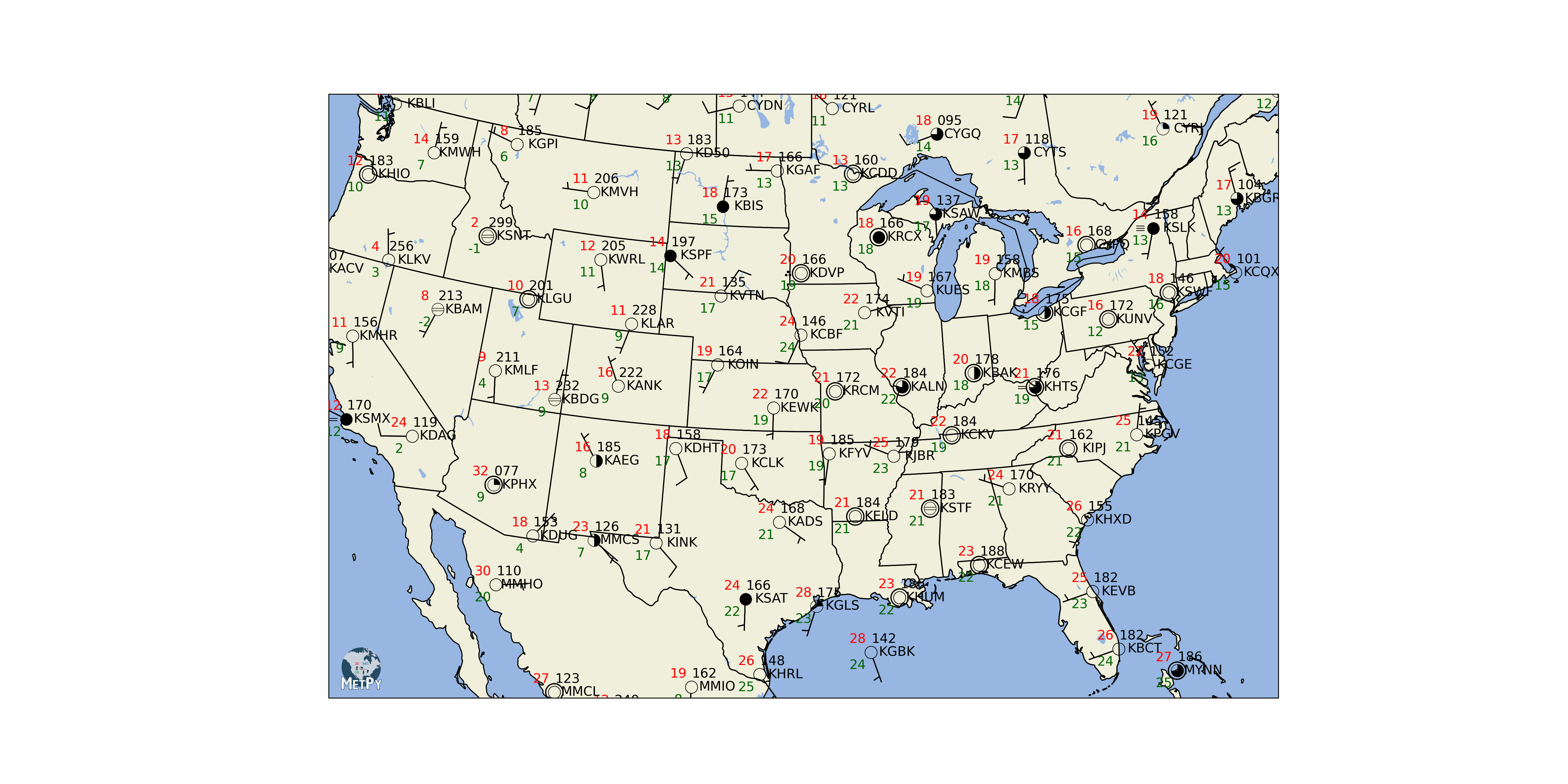
Example of MetPy plotting tools
Calculations
Meteorology also has a common set of calculations that everyone ends up programming themselves. This is error-prone and a huge duplication of work. MetPy contains a set of well-tested calculations that is continually growing in an effort to be at feature parity with other legacy packages such as GEMPAK.
File I/O
Finally, there are a number of odd file formats in the meteorological community. MetPy has incorporated a set of readers to help you deal with file formats that you may encounter during your research, including working with many xarray functions for data organization.
Units and MetPy
Early in our scientific careers we all learn about the importance of paying attention to units in our calculations. Unit conversions can still get the best of us and have caused more than one major technical disaster, including the crash and complete loss of the $327 million Mars Climate Orbiter.
MetPy uses the pint library and a custom unit registry to help prevent unit mistakes in calculations. That means that every quantity you pass to MetPy should have units attached, just like if you were doing the calculation on paper. Attaching units is easy, simply multiply (*) the magnitude by the units in the format units.___.
# Import the MetPy unit registry
from metpy.units import units
length = 10.4 * units.inches
width = 20 * units.meters
print(length, width)10.4 inch 20 meter
You can also use tab completion to see what units are available in the units registry.
Let’s now attempt a rectangular area calculation with the above measurements. Multiplying length and width, we’ll get an area in return with units attached.
area = length * width

print(area)
208.0 inch * meter
That’s great, now we have an area, but it is not in a very useful unit...
MetPy can save you the headache of looking up conversions and maintaining high precision with the .to() method. You have the option of converting the individual measurements or the final area calculation. While you won’t see m in the units list, we can parse complex/compound units as strings:
area.to('m^2')Which outputs the correct units for velocity?
a = 10 * units.m / 20 * units.s
b = 10 * units.m / (20 * units.s)
Temperature
In meteorology, we frequently use three different measurements systems for temperature. We often get temperature in Kelvin from model output, but may want to report temperature for communication purposes in Celsius or Fahrenheit. To convert from one unit of temperature to another, we apply a conversion equation such as:
These conversions are straightforward for simple one to one calculations. Where we run into trouble is when we refer to changes in temperature from one unit system to another. Temperature is a non-multiplicative unit - they are in a system with a reference point. That means that not only is there a scaling factor (9/5), but also an offset (32). This makes the math and unit book-keeping a little more complex.
Imagine running a numerical model that tests the effect of surface temperature on cloud cover. Let’s say we want to increase the baseline surface temperature of 290 K by 8 degrees Celsius. There may be many ways you can think of to complete this operation, so let’s test a few methods:
Imagine adding 10 degrees Celsius to 100 degrees Celsius. Is the answer 110 degrees Celsius or 383.15 degrees Celsius (283.15 K + 373.15 K)? That’s why there are delta degrees units in the unit registry for offset units. For more examples and explanation you can watch MetPy Monday #13.
# Starting simple, try adding 8 degrees C to 290 K
290 * units.kelvin + 8 * units.degC
---------------------------------------------------------------------------
OffsetUnitCalculusError Traceback (most recent call last)
Cell In[5], line 2
1 # Starting simple, try adding 8 degrees C to 290 K
----> 2 290 * units.kelvin + 8 * units.degC
File ~/projects/2026-ams-studentconference/.pixi/envs/default/lib/python3.14/site-packages/pint/facets/plain/quantity.py:874, in PlainQuantity.__add__(self, other)
871 if isinstance(other, datetime.datetime):
872 return self.to_timedelta() + other
--> 874 return self._add_sub(other, operator.add)
File ~/projects/2026-ams-studentconference/.pixi/envs/default/lib/python3.14/site-packages/pint/facets/plain/quantity.py:101, in check_implemented.<locals>.wrapped(self, *args, **kwargs)
99 elif isinstance(other, list) and other and isinstance(other[0], type(self)):
100 return NotImplemented
--> 101 return f(self, *args, **kwargs)
File ~/projects/2026-ams-studentconference/.pixi/envs/default/lib/python3.14/site-packages/pint/facets/plain/quantity.py:851, in PlainQuantity._add_sub(self, other, op)
849 units = other._units
850 else:
--> 851 raise OffsetUnitCalculusError(self._units, other._units)
853 return self.__class__(magnitude, units)
OffsetUnitCalculusError: Ambiguous operation with offset unit (kelvin, degree_Celsius). See https://pint.readthedocs.io/en/stable/user/nonmult.html for guidance.Notice that this fails with error "Ambiguous operation with offset unit" because we cannot add two units with offset reference points.
Instead, we must look again at the problem we are trying to solve: Increase 290 K by 8 degrees Celsius. In this case, the 8 degrees Celsius is not a single temperature measurement, it is a representation of temperature change. On the Kelvin scale, we increase the starting temperature by an equivalent of 8 degrees Celsius, i.e. 8 degrees Celsius.
MetPy (and pint) have a special unit to complete these kinds of calculations, delta_degC. Let’s try our calculation again and find our resulting surface temperature:
290 * units.kelvin + 8 * units.delta_degCAbsolute temperature scales like Kelvin and Rankine do not have an offset and therefore can be used in addition/subtraction without the need for a delta verion of the unit. For example,
>> 273 * units.kelvin + 10 * units.kelvin
>> 283 kelvin
>> 273 * units.kelvin - 10 * units.kelvin
>> 263 kelvin
MetPy Constants
Another common place that problems creep into scientific code is the value of constants. Can you reproduce someone else’s computations from their paper? Probably not unless you know the value of all of their constants. Was the radius of the earth 6000 km, 6300km, 6371 km, or was it actually latitude dependent?
MetPy has a set of constants that can be easily accessed and make your calculations reproducible. You can view a full table in the docs, look at the module docstring with metpy.constants? or checkout what’s available with tab completion.
import metpy.constants as mpconst
import numpy as npmpconst.earth_avg_radiusmpconst.dry_air_molecular_weightYou may also notice in the table that most constants have a short name as well that can be used:
mpconst.Rempconst.Mdmpconst.gamma_dThese constants can be plugged directly into equations to preserve precision. For example, as in the ideal gas law:
# Set density (rho) and virtual temperature (Tv) example values
rho = 1.18 * units('kg/m^3')
Tv = 296 * units.K

# Calculate pressure (P)
P = rho * mpconst.Rd * Tv

# Convert to hectopascal (hPa)
print(P.to(units.hPa))
1002.5994764851101 hectopascal
MetPy Calculations
MetPy also encompasses a set of calculations that are common in meteorology (with the goal of have all of the functionality of legacy software like GEMPAK and more). The calculations documentation has a complete list of the calculations in MetPy.
We’ll scratch the surface and show off a few simple calculations here, but will be using many during the workshop.
import metpy.calc as mpcalc
import numpy as np
# Make some fake data for us to work with
np.random.seed(19990503) # So we all have the same data
u = np.random.randint(0, 15, 10) * units('m/s')
v = np.random.randint(0, 15, 10) * units('m/s')
print(u)
print(v)[14.0 2.0 12.0 5.0 3.0 5.0 14.0 8.0 9.0 10.0] meter / second
[6.0 10.0 7.0 11.0 10.0 13.0 2.0 3.0 5.0 0.0] meter / second
Let’s use the wind_direction function from MetPy to calculate wind direction from these values. Remember you can look at the docstring or the website for help.
direction = mpcalc.wind_direction(u, v)
print(direction)
[246.80140948635182 191.30993247402023 239.74356283647072 204.44395478041653 196.69924423399362 201.03751102542182 261.86989764584405 249.44395478041653 240.94539590092285 270.0] degree
For a given unit of mass, the geostrophic wind is a balance between two forces: the Coriolis (CoF) and pressure gradient (PGF) forces
$$CoF = 2 \Omega V sin(\phi)$$ $$PGF = \frac{1}{\rho}\frac{\Delta P}{d}$$
We can solve for the geostrophic wind speed of a unit mass using this equation: $$V_g = \frac{1}{2 \Omega sin(\phi) \rho}\frac{\Delta P}{d}$$
Calculate the geostrophic wind speed in units of $m/s$ for a unit mass with the following parameters: $$P_1 = 500\,mb$$ $$P_2 = 504\,mb$$ $$d = 200\,km$$ $$\phi = 40^{\circ}$$ $$\rho = 0.70\,\frac{kg}{m^3}$$
deltaP = 4 * units.hPa
d = 200 * units.km
sinphi = np.sin(40 * units.degrees)
rho = 0.70 * units('kg/m^3')
vg = (1/(2*mpconst.omega*sinphi*rho))*(deltaP/d)
vg.to('m/s')Without spoiling too much, we might find some tools in MetPy to help in the future too...
import metpy.calc as mpcalc
mpcalc.geostrophic_wind
<function metpy.calc.geostrophic_wind(height, dx=None, dy=None, latitude=None, x_dim=-1, y_dim=-2, *, parallel_scale=None, meridional_scale=None, longitude=None, crs=None)>Though let’s not get too far ahead of ourselves just yet!
A parcel at 60 degrees Fahrenheit is lifted dry adiabatically from the surface to a level of 1500 meters above ground level.
Assuming a dry adiabatic lapse rate of -10 degrees C per 1000 meters, what is the final temperature of the parcel after lifting?
Hint: Remember to group your units and scalar magnitude with parentheses.
Bonus: Assuming a moist adiabatic lapse rate of -6 degrees C per 1000 meters, what is the temperature of the parcel if it continues lifting moist adiabatically an additional 2000 meters? (Final elevation of 3500 meters)
# define lapse rate
dalr = -10 * units.delta_degC / (1000 * units.meters)

# define starting temperature
parcel_t = 60 * units.degF

# lifting
parcel_t = parcel_t + dalr * (1500 * units.meters)
print("Parcel temp after dry adiabatic lift for 1500 m: " + str(parcel_t) + ", " + str(parcel_t.to('degC')))

# Bonus:
malr = -6 * units.delta_degC / (1000 * units.meters)
parcel_t = parcel_t + malr * (2000 * units.meters)
print("Parcel temp after moist adiabatic lift for additional 2000 m: " + str(parcel_t) + ", " + str(parcel_t.to('degC')))
Parcel temp after dry adiabatic lift for 1500 m: 33.0 degree_Fahrenheit, 0.5555555555555998 degree_Celsius
Parcel temp after moist adiabatic lift for additional 2000 m: 11.400000000000002 degree_Fahrenheit, -11.4444444444444 degree_Celsius
More Information
Further Practice
MetPy User Guide: https://
MetPy Example Gallery: https://
Save Your Work
To save any of the files you modified or edited in this session:
Right click on any item in the left-side navigation pane
Select Download
To recreate the Conda environment used for this session on your local computer:
Open a terminal (Linux or MacOS) or Anaconda Prompt (Windows).
Windows users: If Anaconda Prompt does not exist on your computer, Conda is not installed. Proceed with step 2.2.
Confirm that Conda is installed by executing:
conda --version
If Conda is installed, a version number will be returned. Proceed to step 3.
If Conda is not installed, proceed with the installation instructions provided for your operating system at this link, then proceed to step 3.
Download the conda environment used in this workshop. On the link below, Shift + Right Click > Save link as > save the file as environment.yml in a location of your choosing.
https://
raw .githubusercontent .com /Unidata /metpy -ams -2024 /main /environment .yml In your terminal or command prompt, change directories to the location where the environment.yml file was saved.
Set up the course Python environment with the following command.
Note: this will take a few minutes to complete.
conda env create -f environment.yml
Verify that the environment installed correctly by looking for metpy-analysis in your conda environment list
conda env list
To use the new environment, activate the new environment
conda activate metpy-analysis
Launch Jupyter Lab
jupyter lab