Table of Contents
Introduction to Python-AWIPS
Python-AWIPS is a package that provides access to the AWIPS (Advanced Weather Interactive Processing System) data through the EDEX (Environmental Data EXchange) server. AWIPS is a weather display and analysis package developed by the National Weather Service for operational forecasting.
The DataAccessLayer is the primary interface for requesting meteorological data from an EDEX server. It provides methods for:
Discovering what data types are available
Exploring locations (models, sites, etc.)
Finding available parameters and levels
Querying available times
Retrieving the actual data
In this notebook, we’ll walk through the complete workflow from connecting to an EDEX server to getting data into an xarray Dataset that you can use for analysis and visualization.
Connecting to EDEX
The first step is to import the DataAccessLayer and establish a connection to an EDEX server. Unidata provides a publicly accessible cloud EDEX server for training and research purposes.
from awips.dataaccess import DataAccessLayer

# Connect to Unidata's cloud EDEX server
edex_url = "edex-cloud.unidata.ucar.edu"
DataAccessLayer.changeEDEXHost(edex_url)

print(f"Connected to EDEX server: {edex_url}")
Connected to EDEX server: edex-cloud.unidata.ucar.edu
Exploring Available Data Types
The getSupportedDatatypes() method returns a list of all data types available on the connected EDEX server. These represent different categories of meteorological data.
# Get and display all available data types
data_types = DataAccessLayer.getSupportedDatatypes()
data_types.sort()
list(data_types)
['acars',
'airep',
'binlightning',
'bufrmosavn',
'bufrmoseta',
'bufrmosgfs',
'bufrmoshpc',
'bufrmoslamp',
'bufrmosmrf',
'bufrua',
'climate',
'common_obs_spatial',
'dmw',
'gfe',
'gfeeditarea',
'grid',
'ldadmesonet',
'maps',
'modelsounding',
'obs',
'pirep',
'practicewarning',
'profiler',
'radar',
'radar_spatial',
'satellite',
'sfcobs',
'topo',
'warning']Some commonly used data types include:
| Data Type | Description |
|---|---|
grid | Gridded model data (GFS, NAM, RAP, HRRR, etc.) |
obs | Surface observations (METAR) |
satellite | Satellite imagery |
radar | NEXRAD Level 3 radar data |
modelsounding | Model sounding profiles |
bufrua | Upper air observations |
warning | NWS watches, warnings, and advisories |
Creating a Data Request
To request data, we create a new data request object and specify what we want. The workflow typically involves:
Create a new request with
newDataRequest()Set the data type with
setDatatype()Optionally set location, parameters, levels, etc.
For this example, we’ll request grid data, which contains model output like the GFS.
# Create a new data request for grid data
request = DataAccessLayer.newDataRequest()
request.setDatatype("grid")

print(f"Created request for datatype: grid")
Created request for datatype: grid
Exploring Available Data
Before we can request specific data, we need to know what’s available. The DataAccessLayer provides several methods for exploring the data catalog.
Available Locations
For grid data, “locations” correspond to different models or data sources. Use getAvailableLocationNames() to see what’s available.
# Get available locations (models) for grid data
locations = DataAccessLayer.getAvailableLocationNames(request)
locations.sort()
list(locations)
['AK-NAM11',
'BHP-ALPW',
'BLENDED-PCT_TPW-Sat',
'BLENDED-Rain_Rate-Sat',
'BLENDED-TPW-Sat',
'ESTOFS',
'ESTOFS-other',
'ETSS',
'FFG-ALR',
'FFG-FWR',
'FFG-KRF',
'FFG-MSR',
'FFG-ORN',
'FFG-PTR',
'FFG-RHA',
'FFG-RSA',
'FFG-STR',
'FFG-TAR',
'FFG-TIR',
'FFG-TUA',
'GFS1p0',
'GFS20',
'GOES-East_Gridded_Turbulence',
'GOES-West_Gridded_Turbulence',
'GlobalWave',
'HFR-EAST_6KM',
'HFR-EAST_PR_6KM',
'HFR-US_EAST_DELAWARE_1KM',
'HFR-US_EAST_FLORIDA_2KM',
'HFR-US_EAST_NORTH_2KM',
'HFR-US_EAST_SOUTH_2KM',
'HFR-US_EAST_VIRGINIA_1KM',
'HFR-US_HAWAII_1KM',
'HFR-US_HAWAII_2KM',
'HFR-US_HAWAII_6KM',
'HFR-US_WEST_500M',
'HFR-US_WEST_CENCAL_2KM',
'HFR-US_WEST_LOSANGELES_1KM',
'HFR-US_WEST_LOSOSOS_1KM',
'HFR-US_WEST_NORTH_2KM',
'HFR-US_WEST_SANFRAN_1KM',
'HFR-US_WEST_SOCAL_2KM',
'HFR-US_WEST_WASHINGTON_1KM',
'HFR-WEST_6KM',
'HPCqpfNDFD',
'HREF-AK',
'HREF-HI',
'HREF-SJU',
'HREF-US',
'HRRR',
'HRRR-Smoke',
'HiResW-ARW',
'HiResW-ARW-AK',
'HiResW-ARW-GU',
'HiResW-ARW-HI',
'HiResW-ARW-SJU',
'HiResW-FV3',
'HiResW-FV3-AK',
'HiResW-FV3-GU',
'HiResW-FV3-HI',
'HiResW-FV3-SJU',
'LAMP2p5',
'MRMS_0500',
'MRMS_1000',
'MRMS_AK_1000',
'MRMS_CA_0500',
'MRMS_CA_1000',
'MRMS_GU_0500',
'MRMS_HI_0500',
'NAM12',
'NAM40',
'NationalBlend',
'NationalBlendPR',
'RAP13',
'RTMA',
'RTOFS-HudsonBaffin',
'RTOFS-Now-HudsonBaffin',
'RTOFS-Now-WestAtl',
'RTOFS-Now-WestConus',
'RTOFS-WestAtl',
'RTOFS-WestConus',
'SPCGuide',
'SeaIce',
'TPCWindProb',
'URMA25',
'griddednucaps']Some common model identifiers you might see:
| Location Name | Description |
|---|---|
GFS20 | Global Forecast System (20km) |
NAM12 | North American Mesoscale (12km) |
RAP13 | Rapid Refresh (13km) |
HRRR | High Resolution Rapid Refresh |
MRMS_1000 | Multi-Radar Multi-Sensor |
Let’s select the GFS 20km model for our example.
# Set the location (model) we want to use
request.setLocationNames("GFS20")

print("Selected model: GFS20")
Selected model: GFS20
Available Parameters
Now that we’ve specified a model, we can see what parameters (variables) are available.
# Get available parameters for the selected model
params = DataAccessLayer.getAvailableParameters(request)
params.sort()

# Display first 30 parameters (there are many!)
print(f"Total parameters available: {len(params)}")
print("\nFirst 30 parameters:")
list(params[:30])
Total parameters available: 497
First 30 parameters:
['-10C Hgt AGL',
 '-12 to -18C Omega',
 '-12 to -18C Thickness',
 '-12C Hgt',
 '-18C Hgt',
 '-20C Hgt AGL',
 '-30C Hgt AGL',
 '0 to 3km Line Normal Shear Vectors (Left)',
 '0 to 3km Line Normal Shear Vectors (Right)',
 '0-10km Blk Shr Mag',
 '0-10km Blk Shr Vect',
 '0-1km Blk Shr Mag',
 '0-1km Blk Shr Vect',
 '0-1km EHI',
 '0-1km Helicity',
 '0-1km Mixing Ratio',
 '0-1km Moisture Convergence',
 '0-1km Theta-E',
 '0-1km Theta-E Adv',
 '0-1km Wind Streamlines',
 '0-2km Blk Shr Mag',
 '0-2km Blk Shr Vect',
 '0-2km EHI',
 '0-2km Helicity',
 '0-3km Blk Shr Mag',
 '0-3km Blk Shr Vect',
 '0-3km EHI',
 '0-3km Helicity',
 '0-3km LR',
 '0-3km MLCAPE']
Some commonly used parameters include:
| Parameter | Description |
|---|---|
T | Temperature |
GH | Geopotential Height |
RH | Relative Humidity |
Wind | Wind (vector) |
TP | Total Precipitation |
CAPE | Convective Available Potential Energy |
Let’s select Temperature (T) for our example.
# Set the parameter we want
request.setParameters("T")

print("Selected parameter: T (Temperature)")
Selected parameter: T (Temperature)
Available Levels
For 3D data like model output, we also need to specify which vertical level(s) we want. The getAvailableLevels() method shows what’s available.
# Get available levels for the selected parameter
levels = DataAccessLayer.getAvailableLevels(request)

# Display first 20 levels
print(f"Total levels available: {len(levels)}")
print("\nSample levels:")
for lvl in levels[:20]:
    print(f"  {lvl}")
Total levels available: 258
Sample levels:
700.0MB
1000.0FHAG
0.0SFC
2000.0_5000.0FHAG
0.0_3000.0FHAG
2.0FHAG
1000.0_400.0MB
850.0MB
0.0_6000.0FHAG
850.0_300.0MB
250.0MB
500.0MB
925.0MB
700.0_500.0MB
340.0_350.0K
290.0_300.0K
700.0_600.0MB
700.0_300.0MB
320.0Ke
3962.4FHAG
Level notation guide:
| Suffix | Meaning |
|---|---|
MB | Pressure level in millibars |
SFC | Surface |
FHAG | Fixed Height Above Ground (meters) |
BL | Boundary Layer |
TROP | Tropopause |
K | Isentropic (Kelvin) |
Let’s select the surface level (0.0SFC).
# Set the level we want
request.setLevels("0.0SFC")

print("Selected level: 0.0SFC (Surface)")
Selected level: 0.0SFC (Surface)
Working with Times
Model data includes multiple forecast times. Python-AWIPS provides methods to work with these:
getAvailableTimes(request, True)- Returns available run times (initialization times)getAvailableTimes(request)- Returns all available times (run + forecast)getForecastRun(cycle, times)- Returns times for a specific forecast cycle
# Get available forecast cycles (run times)
cycles = DataAccessLayer.getAvailableTimes(request, True)

print(f"Number of available forecast cycles: {len(cycles)}")
print(f"\nMost recent cycle: {cycles[-1]}")
Number of available forecast cycles: 3
Most recent cycle: 2026-01-25 06:00:00
# Get all available times
times = DataAccessLayer.getAvailableTimes(request)

# Get the forecast run for the most recent cycle
fcst_run = DataAccessLayer.getForecastRun(cycles[-1], times)

print(f"Number of forecast times in latest run: {len(fcst_run)}")
print("\nFirst 10 forecast times:")
for t in fcst_run[:10]:
    print(f"  {t.getRefTime()} : {t.getFcstTime()} seconds ({t.getFcstTime()/3600:.0f} hours)")
Number of forecast times in latest run: 24
First 10 forecast times:
2026-01-25 06:00:00.000 : 0 seconds (0 hours)
2026-01-25 06:00:00.000 : 10800 seconds (3 hours)
2026-01-25 06:00:00.000 : 21600 seconds (6 hours)
2026-01-25 06:00:00.000 : 32400 seconds (9 hours)
2026-01-25 06:00:00.000 : 43200 seconds (12 hours)
2026-01-25 06:00:00.000 : 54000 seconds (15 hours)
2026-01-25 06:00:00.000 : 64800 seconds (18 hours)
2026-01-25 06:00:00.000 : 75600 seconds (21 hours)
2026-01-25 06:00:00.000 : 86400 seconds (24 hours)
2026-01-25 06:00:00.000 : 97200 seconds (27 hours)
Retrieving the Data
Now we’re ready to actually retrieve the data. For gridded data, we use getGridData(). This returns a list of grid objects, each containing the data array and metadata.
# Request data for the first forecast time (analysis, 0 hour)
response = DataAccessLayer.getGridData(request, [fcst_run[0]])

print(f"Number of grid objects returned: {len(response)}")
Number of grid objects returned: 1
# Extract information from the first grid object
grid = response[0]

print("Grid Metadata:")
print(f"  Model:     {grid.getLocationName()}")
print(f"  Parameter: {grid.getParameter()}")
print(f"  Level:     {grid.getLevel()}")
print(f"  Unit:      {grid.getUnit()}")
print(f"  Time:      {grid.getDataTime()}")
print(f"  Forecast:  {grid.getDataTime().getFcstTime()/3600:.0f} hours")
Grid Metadata:
Model: GFS20
Parameter: T
Level: 0.0SFC
Unit: K
Time: 2026-01-25 06:00:00 (0)
Forecast: 0 hours
# Get the raw data array and coordinates
data = grid.getRawData()
lons, lats = grid.getLatLonCoords()

print(f"Data shape: {data.shape}")
print(f"Longitude shape: {lons.shape}")
print(f"Latitude shape: {lats.shape}")
print(f"\nData range: {data.min():.2f} to {data.max():.2f} {grid.getUnit()}")
Data shape: (257, 369)
Longitude shape: (257, 369)
Latitude shape: (257, 369)
Data range: 233.54 to 300.34 K
Converting to xarray
While python-awips returns numpy arrays, it’s often more convenient to work with xarray for analysis and visualization. xarray provides labeled dimensions, coordinate-aware operations, and integrates well with other tools like MetPy.
We can create an xarray Dataset from the numpy arrays returned by python-awips.
import xarray as xr
import numpy as np

# Create an xarray DataArray from the grid data
da = xr.DataArray(
    data=data,
    dims=['y', 'x'],
    coords={
        'latitude': (['y', 'x'], lats),
        'longitude': (['y', 'x'], lons),
    },
    attrs={
        'units': grid.getUnit(),
        'long_name': grid.getParameter(),
        'level': str(grid.getLevel()),
        'model': grid.getLocationName(),
        'valid_time': str(grid.getDataTime()),
    },
    name=grid.getParameter()
)

daCreating a Complete Dataset
For a more complete xarray Dataset with proper time coordinates, we can request multiple forecast times and combine them.
from datetime import datetime, timedelta

# Request data for the first 5 forecast times
num_times = 5
response = DataAccessLayer.getGridData(request, fcst_run[:num_times])

# Build arrays for the Dataset
data_list = []
times_list = []

for grid in response:
    data_list.append(grid.getRawData())
    # Parse the time from the grid object
    ref_time = grid.getDataTime().getRefTime()
    fcst_seconds = grid.getDataTime().getFcstTime()
    # Create a proper datetime
    valid_time = datetime.strptime(str(ref_time)[:19], '%Y-%m-%d %H:%M:%S') + timedelta(seconds=fcst_seconds)
    times_list.append(valid_time)

# Stack data into a 3D array (time, y, x)
data_3d = np.stack(data_list, axis=0)

print(f"Combined data shape: {data_3d.shape}")
Combined data shape: (5, 257, 369)
# Create the xarray Dataset
ds = xr.Dataset(
    data_vars={
        grid.getParameter(): (['time', 'y', 'x'], data_3d, {
            'units': grid.getUnit(),
            'long_name': 'Temperature',
            'level': str(grid.getLevel()),
        })
    },
    coords={
        'time': times_list,
        'latitude': (['y', 'x'], lats),
        'longitude': (['y', 'x'], lons),
    },
    attrs={
        'model': grid.getLocationName(),
        'source': 'EDEX via python-awips',
    }
)

dsUsing the xarray Dataset
Now we have a proper xarray Dataset that we can use with all of xarray’s powerful features.
from metpy.units import units

ds = ds.metpy.parse_cf()

ds.T.metpy.units# Select data by time
temp_first = ds['T'].isel(time=0)
print(f"Data at first time step:")
print(f" Valid time: {temp_first.time.values}")
print(f" Shape: {temp_first.shape}")Data at first time step:
Valid time: 2026-01-25T15:00:00.000000
Shape: (257, 369)
# Quick visualization
import matplotlib.pyplot as plt

# Convert from Kelvin to Celsius for plotting
temp_c = ds['T'].isel(time=0).metpy.convert_units('degC')

fig, ax = plt.subplots(figsize=(12, 8))
img = ax.pcolormesh(temp_c.longitude, temp_c.latitude, temp_c, cmap='RdBu_r', shading='auto')
ax.set_xlabel('Longitude')
ax.set_ylabel('Latitude')
ax.set_title(f'GFS Surface Temperature\nValid: {temp_c.metpy.time.dt.strftime("%Y-%m-%d: %H:%MM:%SS")}')
cbar = plt.colorbar(img, ax=ax, label=f'Temperature [{temp_c.metpy.units:~P}]')
plt.show()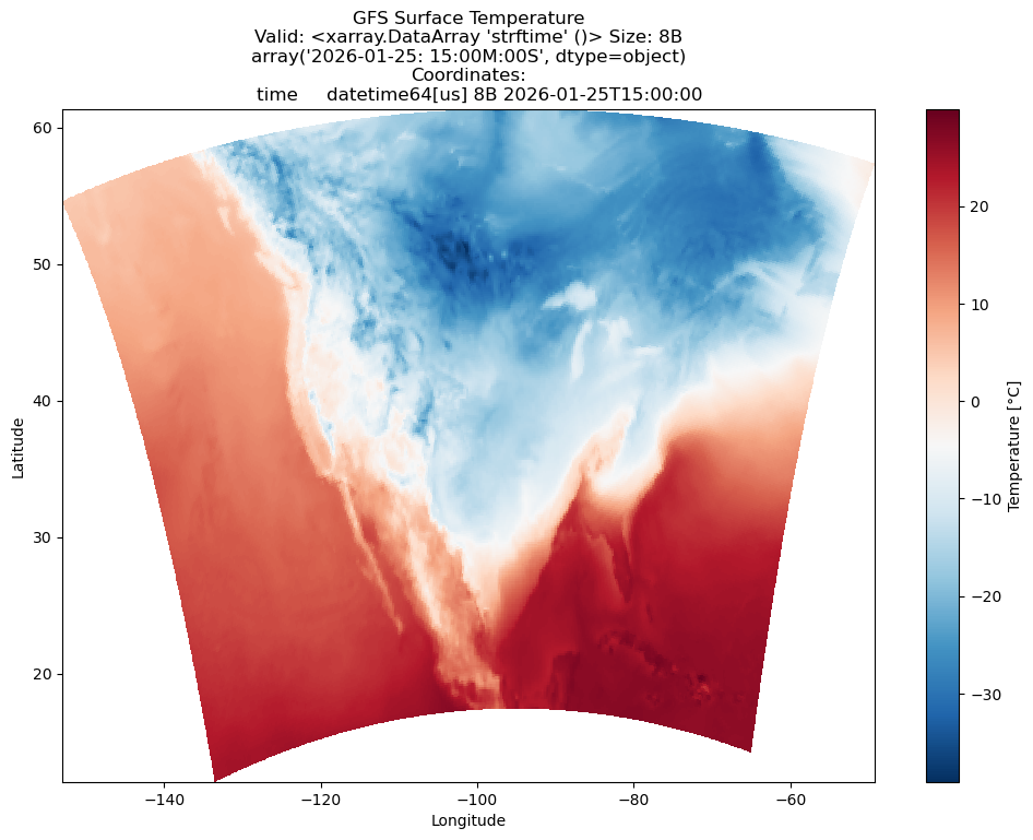
Summary
In this notebook, we learned how to:
Connect to an EDEX server using
DataAccessLayer.changeEDEXHost()Explore available data types with
getSupportedDatatypes()Create a data request with
newDataRequest()and configure itDiscover available locations, parameters, and levels
Query available times and forecast runs
Retrieve data with
getGridData()Convert the data to an xarray Dataset for analysis
Key DataAccessLayer Methods
| Method | Purpose |
|---|---|
changeEDEXHost(url) | Connect to an EDEX server |
getSupportedDatatypes() | List available data types |
newDataRequest() | Create a new request object |
getAvailableLocationNames(request) | Get available locations/models |
getAvailableParameters(request) | Get available parameters |
getAvailableLevels(request) | Get available vertical levels |
getAvailableTimes(request) | Get available times |
getForecastRun(cycle, times) | Get times for a specific run |
getGridData(request, times) | Retrieve gridded data |
getGeometryData(request, times) | Retrieve point/geometry data |