SkewT and Hodograph

Upper Air and the Skew-T Log-P
Unidata Python Workshop
Questions
- Where can upper air data be found and what format is it in?
- How can I obtain upper air data programatically?
- How can MetPy be used to make a Skew-T Log-P diagram and associated fiducial lines?
- How are themodynamic calculations performed on upper-air data?
Table of Contents
1. Obtain upper air data
Overview
Upper air observations are generally reported as a plain text file in a tabular format that represents the down sampled raw data transmitted by the rawinsonde. Data are reported an mandatory levels and at levels of significant change. An example of sounding data may look like this:
-----------------------------------------------------------------------------
   PRES   HGHT   TEMP   DWPT   RELH   MIXR   DRCT   SKNT   THTA   THTE   THTV
    hPa     m      C      C      %    g/kg    deg   knot     K      K      K
-----------------------------------------------------------------------------
 1000.0    270
  991.0    345   -0.3   -2.8     83   3.15      0      0  273.6  282.3  274.1
  984.0    403   10.2   -7.8     27   2.17    327      4  284.7  291.1  285.0
  963.0    581   11.8   -9.2     22   1.99    226     17  288.0  294.1  288.4
  959.7    610   11.6   -9.4     22   1.96    210     19  288.1  294.1  288.5
Data are available to download from the University of Wyoming archive, the Iowa State archive, and the Integrated Global Radiosonde Archive (IGRA). There is no need to download data manually. We can use the siphon library (also developed at Unidata) to request and download these data. Be sure to checkout the documentation on all of siphon's capabilities.
Getting our data
First, we need to create a datetime object that has the time of observation we are looking for. We can then request the data for a specific station. Note that if you provide an invalid time or station where no sounding data are present you will receive an error.
# Create a datetime for our request - notice the times are from laregest (year) to smallest (hour)
from datetime import datetime
request_time = datetime(1999, 5, 3, 12)
# Store the station name in a variable for flexibility and clarity
station = 'OUN'
# Import the Wyoming simple web service and request the data
# Don't worry about a possible warning from Pandas - it's related to our handling of units
from siphon.simplewebservice.wyoming import WyomingUpperAir
df = WyomingUpperAir.request_data(request_time, station)
# Let's see what we got in return
df.head()
We got a Pandas dataframe back, which is great. Sadly, Pandas does not play well with units, so we need to attach units and make some other kind of data structure. We've provided a helper function for this - it takes the dataframe with our special .units attribute and returns a dictionary where the keys are column (data series) names and the values are united arrays. This means we can still use the dictionary access syntax and mostly forget that it is not a data frame any longer.
Fist, let's look at the special attribute siphon added:
df.units
Now let's import the helper and the units registry from MetPy and get units attached.
from metpy.units import pandas_dataframe_to_unit_arrays, units
sounding = pandas_dataframe_to_unit_arrays(df)
sounding
2.Make a Skew-T
Now that we have data, we can actually start making our Skew-T Log-P diagram. This consists of:
- Import matplotlib
- Importing the SkewT object
- Creating a figure
- Creating a SkewT object based upon that figure
- Plotting our data
import matplotlib.pyplot as plt
from metpy.plots import SkewT
%matplotlib inline
# Create a new figure. The dimensions here give a good aspect ratio
fig = plt.figure(figsize=(10, 10))
skew = SkewT(fig)

# Plot the data using normal plotting functions, all of the transforms
# happen in the background!
skew.plot(sounding['pressure'], sounding['temperature'], color='tab:red')
skew.ax.set_ylim(1050,100)
skew.ax.set_xlim(-50,20)
# Redisplay the figure
fig

# Plot a isotherm using axvline (axis vertical line)
skew.ax.axvline(0 * units.degC, color='cyan', linestyle='--')

# Redisplay the figure
fig

- Download your own data using the Wyoming upper-air archive. Have a look at the documentation to help get started.
- Attach units using the unit helper.
# Import the Wyoming simple web service upper air object
# YOUR CODE GOES HERE
# Create the datetime and station variables you'll need
# YOUR CODE GOES HERE
# Make the request for the data - assign it to a dataframe called my_df
# YOUR CODE GOES HERE
# Attach units to the data - assign it to the variable my_sounding
# YOUR CODE GOES HERE
# %load solutions/skewt_get_data.py

# Cell content replaced by load magic replacement.
# Import the Wyoming simple web service upper air object
from siphon.simplewebservice.wyoming import WyomingUpperAir

# Create the datetime and station variables you'll need
request_time = datetime(2011, 4, 14, 18)
station = 'OUN'

# Make the request for the data
my_df = WyomingUpperAir.request_data(request_time, station)

# Attach units to the data
my_sounding = pandas_dataframe_to_unit_arrays(my_df)
- Make a figure and SkewT object.
- Plot the temperature and dewpoint in red and green lines.
- Set the axis limits to sensible limits with set_xlim and set_ylim.
# Make a figure called my_fig

# Make a SkewT object called my_skew

# Plot the temperature and dewpoint
# %load solutions/skewt_make_figure.py

# Cell content replaced by load magic replacement.
# Make a figure
my_fig = plt.figure(figsize=(10, 10))

# Make a SkewT object
my_skew = SkewT(my_fig)

# Plot the temperature and dewpoint
my_skew.plot(my_sounding['pressure'], my_sounding['temperature'], linewidth=2, color='tab:red')
my_skew.plot(my_sounding['pressure'], my_sounding['dewpoint'], linewidth=2, color='tab:blue')

- Plot wind barbs using the plot_barbs method of the SkewT object.
- Add the fiducial lines for dry adiabats, moist adiabats, and mixing ratio lines using the plot_dry_adiabats(), plot_moist_adiabats(), plot_mixing_lines() functions.
# Plot wind barbs

# Add dry adiabats

# Add moist adiabats

# Add mixing ratio lines

# Redisplay figure
# %load solutions/skewt_wind_fiducials.py

# Cell content replaced by load magic replacement.
# Plot wind barbs
my_skew.plot_barbs(my_sounding['pressure'], my_sounding['u_wind'], my_sounding['v_wind'])

# Add dry adiabats
my_skew.plot_dry_adiabats()

# Add moist adiabats
my_skew.plot_moist_adiabats()

# Add mixing ratio lines
my_skew.plot_mixing_lines()

# Redisplay figure
my_fig

3.Thermodynamics
Using MetPy's calculations functions we can calculate thermodynamic paramters like LCL, LFC, EL, CAPE, and CIN. Let's start off with the LCL.
# Add the dewpoint line to our plot we were working with
skew.plot(sounding['pressure'], sounding['dewpoint'], linewidth=2, color='tab:blue')
# Get our basic plot we were working with ready to plot new things on

# Set some good axis limits
skew.ax.set_xlim(-60, 30)
skew.ax.set_ylim(1000, 100)

# Add relevant fiducial lines
skew.plot_dry_adiabats()
skew.plot_moist_adiabats()
skew.plot_mixing_lines()

fig

import metpy.calc as mpcalc
lcl_pressure, lcl_temperature = mpcalc.lcl(sounding['pressure'][0],
                                           sounding['temperature'][0],
                                           sounding['dewpoint'][0])
print(lcl_pressure, lcl_temperature)
We can this as a point on our sounding using the scatter method.
skew.ax.axhline(y=lcl_pressure, color='k', linewidth=0.75)
fig

We can also calculate the ideal parcel profile and plot it.
sounding['profile'] = mpcalc.parcel_profile(sounding['pressure'], sounding['temperature'][0], sounding['dewpoint'][0])
print(sounding['profile'])
# Plot the profile
skew.plot(sounding['pressure'], sounding['profile'], color='black')

# Redisplay the figure
fig

- Calculate the LFC and EL for the sounding.
- Plot them as horizontal line markers.
# Calculate the LFC
# YOUR CODE GOES HERE

# Calculate the EL
# YOUR CODE GOES HERE
# Create a new figure and SkewT object
fig = plt.figure(figsize=(10, 10))
skew = SkewT(fig)

# Plot the profile and data
skew.plot(sounding['pressure'], sounding['profile'], color='black')
skew.plot(sounding['pressure'], sounding['temperature'], color='tab:red')
skew.plot(sounding['pressure'], sounding['dewpoint'], color='tab:blue')

# Plot the LCL, LFC, and EL as horizontal lines
# YOUR CODE GOES HERE

# Set axis limits
skew.ax.set_xlim(-60, 30)
skew.ax.set_ylim(1000, 100)

# Add fiducial lines
skew.plot_dry_adiabats()
skew.plot_moist_adiabats()
skew.plot_mixing_lines()

# %load solutions/skewt_thermo.py

# Cell content replaced by load magic replacement.
# Get data for the sounding
df = WyomingUpperAir.request_data(datetime(1999, 5, 3, 12), 'OUN')

# Calculate the ideal surface parcel path
sounding['profile'] = mpcalc.parcel_profile(sounding['pressure'],
                                            sounding['temperature'][0],
                                            sounding['dewpoint'][0]).to('degC')

# Calculate the LCL
lcl_pressure, lcl_temperature = mpcalc.lcl(sounding['pressure'][0],
                                           sounding['temperature'][0],
                                           sounding['dewpoint'][0])

# Calculate the LFC
lfc_pressure, lfc_temperature = mpcalc.lfc(sounding['pressure'],
                                           sounding['temperature'],
                                           sounding['dewpoint'])

# Calculate the EL
el_pressure, el_temperature = mpcalc.el(sounding['pressure'],
                                        sounding['temperature'],
                                        sounding['dewpoint'])

# Create a new figure and SkewT object
fig = plt.figure(figsize=(10, 10))
skew = SkewT(fig)

# Plot the profile and data
skew.plot(sounding['pressure'], sounding['profile'], color='black')
skew.plot(sounding['pressure'], sounding['temperature'], color='tab:red')
skew.plot(sounding['pressure'], sounding['dewpoint'], color='tab:blue')

# Plot the LCL, LFC, and EL as horizontal markers
if lcl_pressure:
    skew.ax.plot(lcl_temperature, lcl_pressure, marker="_", color='orange', markersize=30, markeredgewidth=3)

if lfc_pressure:
    skew.ax.plot(lfc_temperature, lfc_pressure, marker="_", color='brown', markersize=30, markeredgewidth=3)

if el_pressure:
    skew.ax.plot(el_temperature, el_pressure, marker="_", color='blue', markersize=30, markeredgewidth=3)

# Set axis limits
skew.ax.set_xlim(-60, 30)
skew.ax.set_ylim(1000, 100)

# Add fiducial lines
skew.plot_dry_adiabats()
skew.plot_moist_adiabats()
skew.plot_mixing_lines()

- Use the function surface_based_cape_cin in the MetPy calculations module to calculate the CAPE and CIN of this sounding. Print out the values.
- Using the methods shade_cape and shade_cin on the SkewT object, shade the areas representing CAPE and CIN.
# Calculate surface based cape/cin
# YOUR CODE GOES HERE

# Print CAPE and CIN
# YOUR CODE GOES HERE
# Shade CAPE
# YOUR CODE GOES HERE

# Shade CIN
# YOUR CODE GOES HERE

# Redisplay the figure
fig
# %load solutions/skewt_cape_cin.py
# Cell content replaced by load magic replacement.
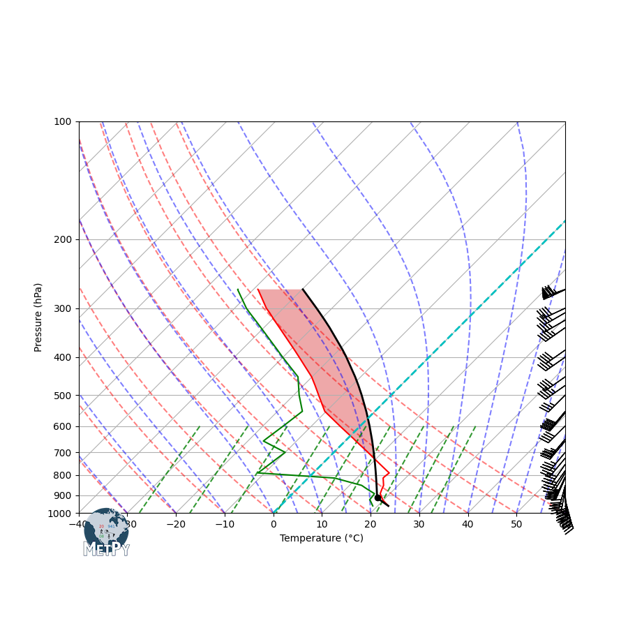
# Calculate surface based cape/cin
surface_cape, surface_cin = mpcalc.surface_based_cape_cin(sounding['pressure'],
sounding['temperature'],
sounding['dewpoint'])
# Print CAPE and CIN
print('CAPE: {}\tCIN: {}'.format(surface_cape, surface_cin))
# Shade CAPE
skew.shade_cape(sounding['pressure'],
sounding['temperature'],
sounding['profile'])
# Shade CIN
skew.shade_cin(sounding['pressure'],
sounding['temperature'],
sounding['profile'])
# Redisplay the figure
fig

4.Plotting a Hodograph
Hodographs are a great way to look at wind shear - they are created by drawing wind vectors, all starting at the origin of a plot, and the connecting the vector tips. They are often thought of as a polar plot where the range rings (lines of constant radius) represent speed and the angle representes the compass angle of the wind.
In MetPy we can create a hodograph in a similar way to a skew-T - we create a hodograph object and attach it to an axes.
# Import the hodograph class
from metpy.plots import Hodograph
# Make a figure and axis
fig, ax = plt.subplots(1, 1, figsize=(6, 6))

# Create a hodograph
h = Hodograph(ax, component_range=60.)

# Add "range rings" to the plot
h.add_grid(increment=20)

# Plot the wind data
h.plot(sounding['u_wind'], sounding['v_wind'], color='tab:red')

We can even add wind vectors, which is helpful for learning/teaching hodographs.
# Add vectors
h.wind_vectors(sounding['u_wind'], sounding['v_wind'])

# Redisplay figure
fig

This is great, but we generally don't care about wind shear for the entire sounding. Let's say we want to view it in the lowest 10km of the atmosphere. We can do this with the powerful, but complex get_layer function. Let's get a subset of the u-wind, v-wind, and windspeed.
(_, u_trimmed, v_trimmed,
 speed_trimmed, height_trimmed) = mpcalc.get_layer(sounding['pressure'],
                                                   sounding['u_wind'],
                                                   sounding['v_wind'],
                                                   sounding['speed'],
                                                   sounding['height'],
                                                   heights=sounding['height'],
                                                   depth=10 * units.km)
Let's make the same hodograph again, but we'll also color the line by the value of the windspeed and we'll use the trimmed data we just created.
from metpy.plots import colortables
import numpy as np
fig, ax = plt.subplots(1, 1, figsize=(6, 6))

h = Hodograph(ax, component_range=60.)
h.add_grid(increment=20)

norm, cmap = colortables.get_with_range('ir_rgbv', np.nanmin(speed_trimmed.m),
                                        np.nanmax(speed_trimmed.m))

h.plot_colormapped(u_trimmed, v_trimmed, speed_trimmed,
                   cmap=cmap, norm=norm)
h.wind_vectors(u_trimmed[::3], v_trimmed[::3])

- Make a variable to hold the height above ground level (subtract the surface height from the heights in the sounding).
- Make an list of boundary values that we'll use to segment the hodograph from 0-1, 1-3, 3-5, and 5-8 km. (Hint the array should have one more value than the number of segments desired.)
- Make a list of colors for each segment.
# Calculate the height above ground level (AGL)
# YOUR CODE GOES HERE
# Make an array of segment boundaries - don't forget units!
# YOUR CODE GOES HERE
# Make a list of colors for the segments
# YOUR CODE GOES HERE
# %load solutions/hodograph_preprocessing.py

# Cell content replaced by load magic replacement.
# Calculate the height above ground level (AGL)
sounding['height_agl'] = sounding['height'] - sounding['height'][0]

# Make an array of segment boundaries - don't forget units!
boundaries = [0, 1, 3, 5, 8] * units.km

# Make a list of colors for the segments
colors = ['tab:red', 'tab:green', 'tab:blue', 'tab:olive']
- Make a new figure and hodograph object.
- Using the bounds and colors keyword arguments to plot_colormapped create the segmented hodograph.
- BONUS: Add a colorbar!
# Create figure/axis
# YOUR CODE GOES HERE

# Create a hodograph object/fiducial lines
# YOUR CODE GOES HERE

# Plot the data
# YOUR CODE GOES HERE

# BONUS - add a colorbar
# YOUR CODE GOES HERE
# %load solutions/hodograph_segmented.py

# Cell content replaced by load magic replacement.
# Create figure/axis
fig, ax = plt.subplots(1, 1, figsize=(6, 6))

# Create a hodograph object/fiducial lines
h = Hodograph(ax, component_range=60.)
h.add_grid(increment=20)

# Plot the data
l = h.plot_colormapped(sounding['u_wind'],
                       sounding['v_wind'],
                       sounding['height_agl'],
                       bounds=boundaries, colors=colors)

# BONUS - add a colorbar
plt.colorbar(l)

5.Advanced Layout
This section is meant to show you some fancy matplotlib to make nice Skew-T/Hodograph combinations. It's a good starting place to make your custom plot for your needs.
# Get the data we want
df = WyomingUpperAir.request_data(datetime(1998, 10, 4, 0), 'OUN')
sounding = pandas_dataframe_to_unit_arrays(df)
# Calculate thermodynamics
lcl_pressure, lcl_temperature = mpcalc.lcl(sounding['pressure'][0],
                                           sounding['temperature'][0],
                                           sounding['dewpoint'][0])

lfc_pressure, lfc_temperature = mpcalc.lfc(sounding['pressure'],
                                           sounding['temperature'],
                                           sounding['dewpoint'])

el_pressure, el_temperature = mpcalc.el(sounding['pressure'],
                                        sounding['temperature'],
                                        sounding['dewpoint'])

parcel_profile = mpcalc.parcel_profile(sounding['pressure'],
                                       sounding['temperature'][0],
                                       sounding['dewpoint'][0])
# Some new imports
import matplotlib.gridspec as gridspec
from mpl_toolkits.axes_grid1.inset_locator import inset_axes
from metpy.plots import add_metpy_logo
# Make the plot
# Create a new figure. The dimensions here give a good aspect ratio
fig = plt.figure(figsize=(9, 9))
add_metpy_logo(fig, 630, 80, size='large')

# Grid for plots
gs = gridspec.GridSpec(3, 3)
skew = SkewT(fig, rotation=45, subplot=gs[:, :2])

# Plot the sounding using normal plotting functions, in this case using
# log scaling in Y, as dictated by the typical meteorological plot
skew.plot(sounding['pressure'], sounding['temperature'], 'tab:red')
skew.plot(sounding['pressure'], sounding['dewpoint'], 'tab:green')
skew.plot(sounding['pressure'], parcel_profile, 'k')

# Mask barbs to be below 100 hPa only
mask = sounding['pressure'] >= 100 * units.hPa
skew.plot_barbs(sounding['pressure'][mask], sounding['u_wind'][mask], sounding['v_wind'][mask])
skew.ax.set_ylim(1000, 100)

# Add the relevant special lines
skew.plot_dry_adiabats()
skew.plot_moist_adiabats()
skew.plot_mixing_lines()

# Shade areas
skew.shade_cin(sounding['pressure'], sounding['temperature'], parcel_profile)
skew.shade_cape(sounding['pressure'], sounding['temperature'], parcel_profile)

# Good bounds for aspect ratio
skew.ax.set_xlim(-25, 30)

if lcl_pressure:
    skew.ax.plot(lcl_temperature, lcl_pressure, marker="_", color='tab:orange', markersize=30, markeredgewidth=3)

if lfc_pressure:
    skew.ax.plot(lfc_temperature, lfc_pressure, marker="_", color='tab:brown', markersize=30, markeredgewidth=3)

if el_pressure:
    skew.ax.plot(el_temperature, el_pressure, marker="_", color='tab:blue', markersize=30, markeredgewidth=3)

# Create a hodograph
agl = sounding['height'] - sounding['height'][0]
mask = agl <= 10 * units.km
intervals = np.array([0, 1, 3, 5, 8]) * units.km
colors = ['tab:red', 'tab:green', 'tab:blue', 'tab:olive']
ax = fig.add_subplot(gs[0, -1])
h = Hodograph(ax, component_range=30.)
h.add_grid(increment=10)
h.plot_colormapped(sounding['u_wind'][mask], sounding['v_wind'][mask], agl[mask], intervals=intervals, colors=colors)
