GEMPAK Online Tutorial
7. Gridded Data Mapping
Gridded data may be obtained from numerical model output, or by performing objective analysis on surface or sounding data sets using the OA programs. For now, we will deal with data that is already in gridded form. Later we will see what goes in to converting surface and upper air data into grid files, and learn about the various models available for ingest via the LDM.
Grid Data Types
Gridded data assumes one of two forms:
- Scalar data - possess only magnitude (handled by the program
gdcntr)
- Vector data - comprised of both magnitude and direction (handled by
gdstream and gdwind)
The program gdplot2 is designed to handle both scalar and vector data. Think of gdplot2 as a combination of the capabilities offered by gdcntr, gdstream and gdwind in one program.
Before we look at the GD plotting programs, we have to familiarize ourselves with a very useful program called gdinfo.
GDINFO - Grid Info
gdinfo lists information about the navigation and fields stored within a GEMPAK grid file.
GDFILE    Grid file
LSTALL    Full list flag
OUTPUT    Output device/filename
GDATTIM   Grid date/time
GLEVEL    Grid level
GVCORD    Grid vertical coordinate
GFUNC     Scalar grid
Let's run gdinfo for the first time to load the default Hurricane Bob grid:
gdinfo
GDFILE    Grid file                         $GEMPAK/data/hrcbob.grd
LSTALL    Full list flag                    YES
OUTPUT    Output device/filename            T
GDATTIM   Grid date/time                    LAST
GLEVEL    Grid level                        500
GVCORD    Grid vertical coordinate          PRES
GFUNC     Scalar grid                       TMPC
Parameters requested: GDFILE,LSTALL,OUTPUT,GDATTIM,GLEVEL,GVCORD,GFUNC.
GEMPAK-GDINFO>r
Grid Navigation
Before listing the requested grids, gdinfo will print out the full pathname of the grid file, the grid navigation, analysis block, and number of grids in the file:
 GRID FILE: /Users/gempak/GEMPAK6.7.0/gempak/data/hrcbob.grd

 GRID NAVIGATION:
     PROJECTION:          STR
     ANGLES:                90.0  -105.0     0.0
     GRID SIZE:           53  45
     LL CORNER:               7.65   -133.44
     UR CORNER:              44.29    -23.75

 GRID ANALYSIS BLOCK:
     ANALYSIS TYPE:        BARNES
     DELTAN:               3.750
     DELTAX:               2.110
     DELTAY:               0.833
     GRID AREA:             7.65 -133.44   44.29  -23.75
     EXTEND AREA:           7.65 -133.44   44.29  -23.75
     DATA AREA:             7.65 -133.44   44.29  -23.75

 Number of grids in file:   433

 Maximum number of grids in file:    500
Un oh, what's this?
[GDU 2] Did not find any matching grids.
This is because gdinfo is looking for grid TMPC at 500 mb PRES at GDATTIM = last, but this grid can not be found. Let's set GFUNC = all and GDATTIM = first to see the first grids available:
  NUM       TIME1              TIME2           LEVL1 LEVL2  VCORD PARM
   33     910819/0000F000                        500         PRES TMPK
   34     910819/0000F000                        500         PRES RELH
   36     910819/0000F000                        500         PRES HGHT
   37     910819/0000F000                        500         PRES OMEG
   38     910819/0000F000                        500         PRES UREL
   39     910819/0000F000                        500         PRES VREL
 Note that if only one parameter is entered, the program searches only for that parameter. In the case above, the grid
 TMPC was being searched for but not found. gdinfo does not perform grid parameter conversions!
If GFUNC = all is entered, the program will match all of the parameters in its search. Entering several parameters separated by semicolons will match those parameters only.
Now that we know what grids are available, we can start plotting the data with gdcntr.
Scalar Plotting
GDCNTR Input Parameters
gdcntr draws contour lines through a scalar grid computed
using the GEMPAK grid diagnostic functions.
GDATTIM   Grid date/time
GLEVEL    Grid level
GVCORD    Grid vertical coordinate
GFUNC     Scalar grid
GDFILE    Grid file
CINT      Contour interval/min/max
LINE      Color/type/width/label/smth/fltr/scflg
MAP       Map color/dash/width/filter flag
MSCALE    fgc;bgc;mask/units/lat;hide/values/anch/x;y/ln;wd/freq|text_info|t
TITLE     Title color/line/title
DEVICE    Device|name|x size;y size|color type
SATFIL    Satellite image filename(s)
RADFIL    Radar image filename(s)
IMCBAR    Color/ornt/anch/x;y/ln;wd/freq
PROJ      Map projection/angles/margins|drop flag
GAREA     Graphics area
IJSKIP    Iskp;Istrt;Istp/Jskp;Jstrt;Jstp
CLEAR     Clear screen flag
PANEL     Panel loc/color/dash/width/regn
TEXT      Size/fnt/wdth/brdr/N-rot/just/hw flg
SCALE     Scalar scale / vector scale
LATLON    Line color/dash/width/freq/inc/label/format
HILO      Color/symbol/rng/rad/cnt/intp
HLSYM     HILO txt size/posn/font/wdth/hw
CLRBAR    Color/ornt/anch/x;y/ln;wd/freq|text_info
CONTUR    Subbox/smooth
SKIP      Skip_cntr/skip_plt_x;skip_plt_y
FINT      Fill interval/min/max
FLINE     Fill colors/fill types
CTYPE     Contour type:  C/F
LUTFIL    Enhancement lookup table filename
STNPLT    Txtc/txt attr|marker attr|stnfil#col
Contouring and Filling
Contours may be displayed three different ways:
CTYPE = c draws contour lines using input from CINT and LINE.CTYPE = f draws filled contours using input from FINT and FLINE.CTYPE = f/c draws both contour lines and filled contours.
CINT specifies the contour interval, minimum value, and maximum value separated with slashes:
CINT = contour interval / minimum / maximum / ndigits
Likewise, FINT specified the same intervales, minimum and maximum values for color-filled contours.
Line Type
LINE is the color, line type, line width, line label freqency, smoothing separated by slashes, and flag to suppress small contours. The individual values in each group are separated by semicolons:
colr1;..;colrn/type1;..;typen/width1;..;widthn/labl1;..;labln/smth/fltr
For example:
LINE = 1;2 / 7;8 / 4;5 / 2 / 2
assigns colors 1 and 2 to alternate lines, dashing patterns 7 and 8 to
alternate lines, line widths 4 and 5 to alternate lines, and labels
every other line. Smoothing level 2 is used on all lines.
 If any specification is missing, a default of 1 is used, except for smoothing, which defaults to 0, or no smoothing.
There are ten distinct line types:
- solid
- short dashed
- medium dashed
- long dash short dash
- long dash
- long dash three short dashes
- long dash dot
- long dash three dots
- medium dash dot
- dotted
Exercise #9 (Simple Gridded Contours)
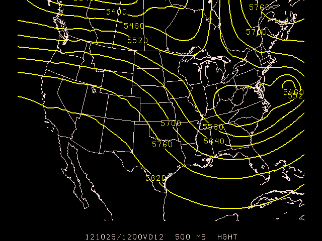
Use gdcntr to plot 500mb heights for last nights 0000 UTC GFS forecast valid at 1200 UTC this morning, using the standard 60 m contour interval.
 GDATTIM  = 0000f12
 GLEVEL   = 500
 GVCORD   = pres
 GFUNC    = hght
 GDFILE   = gfs
 CINT     = 60
 LINE     = 5/1/2
 MAP      = 1
 MSCALE   = 0
 TITLE    = @
 DEVICE   = xw
 SATFIL   =
 RADFIL   =
 IMCBAR   =
 PROJ     = STR/90;-100;0
 GAREA    = us
 IJSKIP   =
 CLEAR    = yes
 PANEL    = 0
 TEXT     = 1
 SCALE    = 999
 LATLON   =
 HILO     =
 HLSYM    =
 CLRBAR   =
 CONTUR   = 3
 SKIP     = 0
 FINT     = 0
 FLINE    = 10-20
 CTYPE    = C
 LUTFIL   =
 STNPLT   =

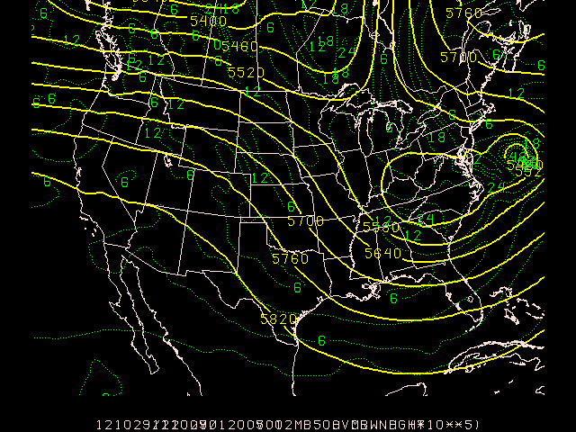
Now overlay 500mb absolute vorticity ontop of the 500mb map we just plotted. Remember the check the CLEAR setting so the graphics area isn't cleared before we plot another layer!
 CLEAR    = no
 GFUNC    = avor(wnd)
 CINT     = 0
 LINE     = 3/10
 TITLE    = 1/-2

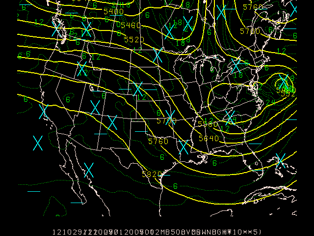
Now mark the vorticity centers the old fashioned way, X's for maximas, -'s for minimas, and run again
hilo = 6;6/X;-
hlsym = 3/2/22/1/hw

Exercise #10 (Color-Fill Grid Contours)
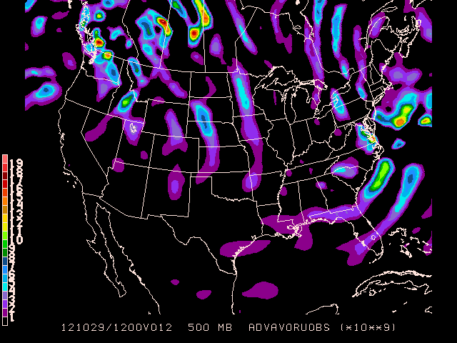
With that we've visualized vorticity advection for this morning's forecast from last night. But why don't we save some work and have GEMPAK compute vorticity advection itself:
clear = y
ctype = f
hilo =
fline = 0;30-7
fint = 1/1
scale = 9
gfunc = adv(avor(wnd),wnd)

GDMAP - Point Data
gdmap plots data computed from GEMPAK grid files on a map.
 GDATTIM  = 0000f12
 GLEVEL   = 500
 GVCORD   = pres
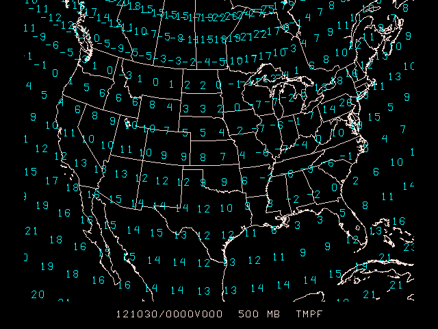
 GFUNC    = tmpf
 GDFILE   = gfs
 GAREA    = us
 IJSKIP   = 2
 COLORS   = 6
 TITLE    = 1/-2
 SCALE    =
 DEVICE   = xw
 PROJ     = STR/90;-100;0
 CLEAR    = y
 TEXT     = 1
 GRDLBL   = 0

Vector Plotting
GDWIND - Wind Vectors
gdwind draws wind barbs or arrows at each grid point of a
vector grid. Vector plots can be drawn for any vector field
computed using the GEMPAK grid diagnostic functions.
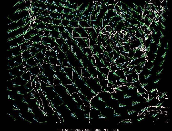
As an example, plot 300 and 700 mb wind barbs
 GDATTIM  = 0000f12
 GLEVEL   = 300
 GVCORD   = pres
 GVECT    = geo
 GDFILE   = gfs
 GAREA    = us
 IJSKIP   = 1
 SATFIL   =
 RADFIL   =
 IMCBAR   = 1
 SKIP     = /-1
 WIND     = bk6
 REFVEC   =
 MAP      = 1
 MSCALE   = 0
 LATLON   =
 PANEL    = 0
 TITLE    = 1
 DEVICE   = xw
 PROJ     = STR/90;-100;0
 CLEAR    = y
 SCALE    =
 TEXT     = 1
 LUTFIL   =
 STNPLT   =
 GEMPAK-GDWIND>r

 CLEAR    = no
 GLEVEL   = 700
 WIND     = bk22
 GEMPAK-GDWIND>r

GDSTREAM - Streamlines
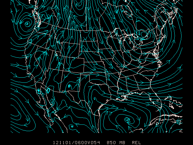
gdstream draws streamlines through any vector grid computed
by the grid diagnostics package. The vector grid is specified
by GVECT.
 GDATTIM  = last
 GLEVEL   = 850
 GVCORD   = pres
 GVECT    = wnd
 GDFILE   = gfs
 GAREA    = us
 IJSKIP   =
 SATFIL   =
 RADFIL   =
 IMCBAR   = 1
 LINE     = 6/1
 MAP      = 1
 MSCALE   = 0
 LATLON   =
 TITLE    = 1
 PANEL    = 0
 TEXT     = 1
 DEVICE   = xw
 PROJ     = STR/90;-100;0
 CLEAR    = y
 WIND     =
 LUTFIL   =
 STNPLT   =
 STREAM   =

In the examples above, we were able to contour layers on top of each other with the CLEAR = no definition. Now we will learn an easier way to display multiple grids on the same map using gdplot2.
Plotting Scalars and Vectors
GDPLOT2 Input Parameters
gdplot2 has the special ability to plot multiple sets of contours, vectors and/or streamlines for each frame.
GDFILE    Grid file
GDATTIM   Grid date/time
GLEVEL    Grid level
GVCORD    Grid vertical coordinate
PANEL     Panel loc/color/dash/width/regn
SKIP      Skip_cntr/skip_plt_x;skip_plt_y
SCALE     Scalar scale / vector scale
GDPFUN    Scalar grid or vector grid function
TYPE      GDPLOT2 function processing type
CONTUR    Subbox/smooth
CINT      Contour interval/min/max
LINE      Color/type/width/label/smth/fltr/scflg
FINT      Fill interval/min/max
FLINE     Fill colors/fill types
HILO      Color/symbol/rng/rad/cnt/intp
HLSYM     HILO txt size/posn/font/wdth/hw
CLRBAR    Color/ornt/anch/x;y/ln;wd/freq|text_info
WIND      Wind symbol/siz/wdth/typ/hdsz
REFVEC    Mag;x;y;txtsiz/font/wdth/HW;labl
TITLE     Title color/line/title
TEXT      Size/fnt/wdth/brdr/N-rot/just/hw flg
CLEAR     Clear screen flag
GAREA     Graphics area
IJSKIP    Iskp;Istrt;Istp/Jskp;Jstrt;Jstp
PROJ      Map projection/angles/margins|drop flag
MAP       Map color/dash/width/filter flag
MSCALE    fgc;bgc;mask/units/lat;hide/values/anch/x;y/ln;wd/freq|text_info|t
LATLON    Line color/dash/width/freq/inc/label/format
DEVICE    Device|name|x size;y size|color type
STNPLT    Txtc/txt attr|marker attr|stnfil#col
SATFIL    Satellite image filename(s)
RADFIL    Radar image filename(s)
IMCBAR    Color/ornt/anch/x;y/ln;wd/freq
LUTFIL    Enhancement lookup table filename
STREAM    lines/arrows/stop/slow/scale
POSN      Position / Text format
COLORS    Color list
MARKER    Marker color/type/size/width/hw
GRDLBL    Grid point label color
FILTER    Filter data factor
Plotting Multiple Fields
Exclamation points ! are used in GDPFUN to delimit multiple overlays of scalar and vector fields. All other parameters (except DEVICE, CLEAR and LUTFIL) may contain exclamation points to delimit specifications for the fields defined by GDPFUN. If any parameter contains more specifications than the maximum number of plots specified in GDPFUN or GDFILE, they will be ignored. Positions between exclamation points may be left blank. Most parameters will replace the blank with the previous value (repeat). A trailing exclamation point will be treated as a blank. If there is no trailing exclamation point, the last specification will be repeated for subsequent plots.
Exercise #11 (Scalars and Vectors)
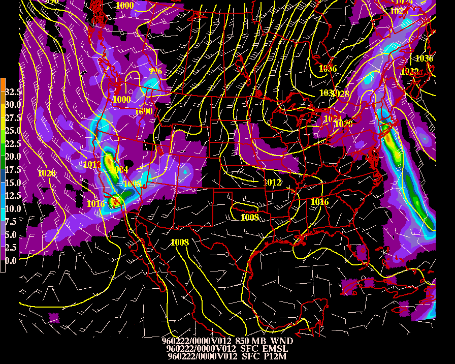
Use gdplot2 to plot 12-hr precipitation color area contours, overlaid with sea level pressure line contours, and 850 mb wind vectors. Use the 12hr forecast fields of the most recent GFS model.
GDPFUN  = p12m      ! emsl      ! wnd
GLEVEL  = 0         ! 0         ! 850
GVCORD  = none      ! none      ! pres
TYPE    = f         ! c         ! b
GAREA   = uslcc
PROJ    = def
CINT    =           ! 4         !
FINT    = 2.5/2.5   !           !
FLINE   = 0;30-7
SCALE   = 0
TITLE   = 1/-1      ! 1/-2      ! 1/-3
GEMPAK-GDPLOT2>r
Each column seperated by exclamation points essentially contains it's own instructions on what to contour or plot and how. gdplot2 eliminates the need to run GEMPAK programs multiple times with the CLEAR = n option.
In this example there are three fields being plotted:
- 12-hour precipitation in mm
GDPFUN = p12m at the surface GLEVEL = 0 with a fill interval of 2.5 mm, beginning at 2.5 mm FINT = 2.5/2.5, each level colored in the range 30-7, with no color drawn for levels lower than 2.5 mm FLINE = 0;30-7.
- sea level pressure
GDPFUN = emsl contoured TYPE = c every 4 millibars CINT = 4.
- 850mb
GLEVEL = 850 wind GDPFUN = wnd barbs TYPE = b.

Later on in the workshop tutorial we will revisit multiple fields plotted on the same map using gdplot2, and get more in depth with shell scripting to make it happen.
GEMPAK Online Tutorial | Next: Grid Diagnostics
![]() Note that if only one parameter is entered, the program searches only for that parameter. In the case above, the grid
Note that if only one parameter is entered, the program searches only for that parameter. In the case above, the grid 