GEMPAK Online Tutorial

8. Grid Diagnostics

GEMPAK possess a robust set of mathmatical and meteorological functions which may be used in the grid programs to generate a wide range of diagnostics.

Formulas can be extended up to 128 characters. When designing complex equations, it is often helpful to develop the equation in pieces, or terms. In these cases, GDDIAG can be used to calculate store the terms, for ultimate use in the final expansion.

When storing grids with GDDIAG, the variable GRDNAM will be used to define a name for the new parameter. If this parameter is left blank, GEMPAK will compose a name based on the variables and functions used in the expression.

In-line Modifiers

Many times, a single GLEVEL, GDATTIM, or even GVCORD is not sufficient for calculating all the quantities in a formula. In these cases we need to use in-line modifiers.

In line expansions allow us to modify the values used for a parameter in a per-variable manner.

The following may be used to specify a value other than that which a variable would obtain if using the values specified in the user interface variables:

^time, @level, %vcord

Additionally, we may need to specify more than 1 value, as in the case of a layer quantity such as thickness between pressure levels, or as in time differences such as the height change of a surface with time.

When we have to specify more than 1 value for a level or time parameter (either in GLEVEL and GDATTIM, or through the in-line modifiers) the values are separated with a color: :.

Multiple Grid Files

When multiple grid files are used, a + character is used in the GDFILE variable to separate the filenames. Then when referencing which file a grid field should be found, the variable is appended with +n, where n is the number of the grid file in the order given in GDFILE.

Remember the batch script we created? Now we're going to modify it perform more complicated grid diagnostics.

Exercise #12 (Grid Diagnostics with Multiple Files and In-line Modifiers)

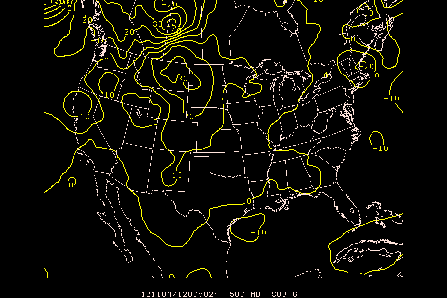
Using the ability to open multiple input files, compare the 24 hour 500mb height forecast from the GFS and ETA models by computing the difference of the height fields.

define two files in GDFILE using +
reference the second of the two files by using the in-line modifier +2

allow CINT = 0 for automatic contouring

   GDATTIM  = f024
   GLEVEL   = 500
   GVCORD   = pres
   GFUNC    = sub(hght,hght+2)
   GDFILE   = eta + gfs
   CINT     = 0
   LINE     = 5
   MAP      = 3/1/1
   TITLE    = 1
   DEVICE   = xw
   SATFIL   =  
   RADFIL   =  
   PROJ     = str/90;-100;0
   GAREA    = us
   CLEAR    = YES
   PANEL    = 0
   TEXT     = 1
   SCALE    = 999
   LATLON   = 0
   HILO     =  
   HLSYM    =
   CLRBAR   = 
   CONTUR   = 3/3
   SKIP     = 0
   FINT     = 
   FLINE    = 
   CTYPE    = c
   LUTFIL   = default
   STNPLT   =  
  GEMPAK-GDCNTR>r

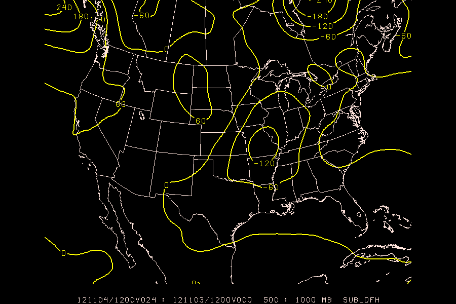
Produce a contour plot of the 1000-500mb change in thickness between the 0 and 24 hour forecast ETA fields.

Use the layer difference function ldf() along with the subtraction function sub(X,Y) (see the GPARM man page for help)

You'll need to specify the exact times for the paramaters used in the calculation (see "in-line modifiers" above).

   GDATTIM  = f000
   GLEVEL   = 500:1000
   GVCORD   = pres
   GFUNC    = sub(ldf(hght^f024),ldf(hght^f000))
   GDFILE   = eta
   CINT     = 60
   LINE     = 5
   MAP      = 1
   TITLE    = 1
   DEVICE   = xw
   SATFIL   = 
   RADFIL   = 
   PROJ     = str/90;-100;0
   GAREA    = us
   CLEAR    = y
   PANEL    = 0
   TEXT     = 1.3/22/1/hw
   SCALE    = 
   LATLON   = 0
   HILO     = 
   HLSYM    = 
   CLRBAR   = 
   CONTUR   = 3/3
   SKIP     = 0
   FINT     = 
   FLINE    = 
   CTYPE    = c
   GEMPAK-GDCNTR>r

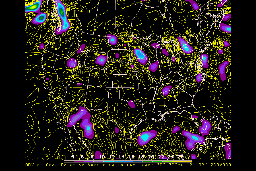
Contour the advection of 500mb geostrophic relative vorticity by the thermal wind in the 300mb to 700mb layer (i.e. Trenberth's Q-G formula).

functions you'll need to use:

advection: adv()
vorticity: vor()
thermal wind: thrm()
use in-line modifiers for hght@300:700 to calculate the thermal wind

you'll need to adjust the contour interval down from 60 (try CINT = 2//2)

   GDATTIM  = f000
   GLEVEL   = 500
   GVCORD   = pres
   GFUNC    = adv(vor(geo),thrm(hght@300:700))
   GDFILE   = eta
   CINT     = 2//2
   LINE     = 5
   MAP      = 6
   TITLE    = 5/-2/ADV of Geo. Relative Vorticity in the layer 300-700mb ~
   DEVICE   = xw
   SATFIL   = 
   RADFIL   = 
   PROJ     = str/90;-100;0
   GAREA    = us
   CLEAR    = y
   PANEL    = 0
   TEXT     = 1.3/22/1/hw
   SCALE    = 
   LATLON   = 0
   HILO     = 
   HLSYM    = 
   CLRBAR   = 1/h/lc/.5/.5;.01
   CONTUR   = 3/3
   SKIP     = 0
   FINT     = 2/4
   FLINE    = 0;30-7
   CTYPE    = c/f
   GEMPAK-GDCNTR>

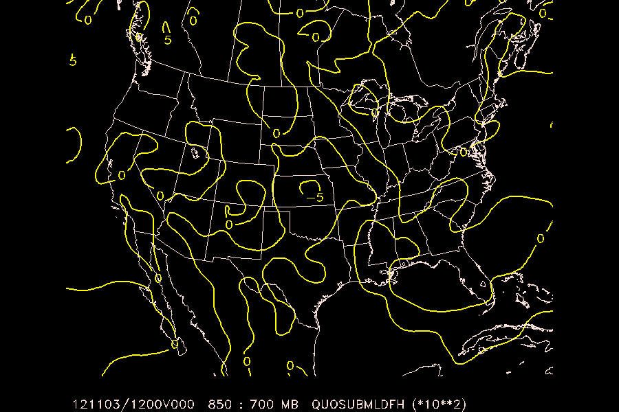
Calculate and plot helicity for the 1000mb - 700mb layer using the formula:

functions you'll need to use:

quotient: quo(X,Y)
subtraction: sub(X,Y)
multiplication: mul(X,Y)
layer difference: ldf()
you'll need to adjust the contour interval to CINT = 5

First we must rewrite the formula for helicity in GEMPAK GPARM notation!

In "psuedocode", the forumla would look like:

      H =  vrel@850 * (urel@700 - urel@1000)/(hght@700 - hght@1000)
         - urel@850 * (vrel@700 - vrel@1000)/(hght@700 - hght@1000)

Substituting ldf() for the hght, urel and vrel differences, and using our GLEVEL = 700:1000 definition:

      H =  vrel@850 * ( ldf(urel) )/( ldf(hght) )
         - urel@850 * ( ldf(vrel) )/( ldf(hght) )

Factoring out the common denominator:

      H = ( vrel@850 * ldf(urel)  - urel@850 * ldf(vrel) )
         % ldf(hght)

Now using the sub(), mul() and qou() mathematical operators:

     H = quo( sub(mul(vrel@850,ldf(urel)),mul(urel@850,ldf(vrel))), ldf(hght) )

So the full entry to GDCNTR would be:

      GEMPAK-GDCNTR>l
      GDATTIM  = f000
      GLEVEL   = 700:1000
      GVCORD   = pres
      GFUNC    = quo(sub(mul(vrel@850,ldf(urel)),mul(urel@850,ldf(vrel))),ldf(hght))
      GDFILE   = eta
      CINT     = 5
      LINE     = 5//2
      MAP      = 1
      TITLE    = 1
      DEVICE   = xw
      SATFIL   = 
      RADFIL   = 
      PROJ     = str/90;-100;0
      GAREA    = us
      CLEAR    = y
      PANEL    = 0
      TEXT     = 1.3/22/1/hw
      SCALE    = 2
      LATLON   = 0
      HILO     = 
      HLSYM    = 
      CLRBAR   = 1/h/lc/.5/.5;.01
      CONTUR   = 3/3
      SKIP     = 0
      FINT     = 2/4
      FLINE    = 0;30-7
      CTYPE    = c
      GEMPAK-GDCNTR>r

GEMPAK Online Tutorial | Next: Grid Interpolation and Transformation