Note
Click here to download the full example code
Cross Section Analysis
The MetPy function metpy.interpolate.cross_section can obtain a cross-sectional slice through
gridded data.
import cartopy.crs as ccrs
import cartopy.feature as cfeature
import matplotlib.pyplot as plt
import numpy as np
import xarray as xr

import metpy.calc as mpcalc
from metpy.cbook import get_test_data
from metpy.interpolate import cross_section
Getting the data
This example uses NARR reanalysis data for 18 UTC 04 April 1987 from NCEI (https://www.ncdc.noaa.gov/data-access/model-data).
We use MetPy’s CF parsing to get the data ready for use, and squeeze down the size-one time dimension.
data = xr.open_dataset(get_test_data('narr_example.nc', False))
data = data.metpy.parse_cf().squeeze()
print(data)
Out:
<xarray.Dataset>
Dimensions:              (isobaric: 29, x: 292, y: 118)
Coordinates:
    time                 datetime64[ns] 1987-04-04T18:00:00
  * isobaric             (isobaric) float64 1e+03 975.0 950.0 ... 125.0 100.0
  * y                    (y) float64 -3.087e+06 -3.054e+06 ... 7.114e+05
  * x                    (x) float64 -3.977e+06 -3.945e+06 ... 5.47e+06
    crs                  object Projection: lambert_conformal_conic
Data variables:
    Temperature          (isobaric, y, x) float32 ...
    Lambert_Conformal    |S1 ...
    lat                  (y, x) float64 ...
    lon                  (y, x) float64 ...
    u_wind               (isobaric, y, x) float32 ...
    v_wind               (isobaric, y, x) float32 ...
    Geopotential_height  (isobaric, y, x) float32 ...
    Specific_humidity    (isobaric, y, x) float32 ...
Define start and end points:
start = (37.0, -105.0)
end = (35.5, -65.0)
Get the cross section, and convert lat/lon to supplementary coordinates:
cross = cross_section(data, start, end)
cross.set_coords(('lat', 'lon'), True)
print(cross)
Out:
<xarray.Dataset>
Dimensions:              (index: 100, isobaric: 29)
Coordinates:
    time                 datetime64[ns] 1987-04-04T18:00:00
  * isobaric             (isobaric) float64 1e+03 975.0 950.0 ... 125.0 100.0
    crs                  object Projection: lambert_conformal_conic
    x                    (index) float64 1.818e+05 2.18e+05 ... 3.712e+06
    y                    (index) float64 -1.454e+06 -1.447e+06 ... -5.573e+05
  * index                (index) int64 0 1 2 3 4 5 6 7 ... 93 94 95 96 97 98 99
    lat                  (index) float64 37.0 37.05 37.11 ... 35.66 35.58 35.5
    lon                  (index) float64 -105.0 -104.6 -104.2 ... -65.39 -65.0
Data variables:
    Temperature          (isobaric, index) float64 287.7 286.9 ... 211.4 211.4
    Lambert_Conformal    |S1 ...
    u_wind               (isobaric, index) float64 -2.729 0.4776 ... 24.6 23.68
    v_wind               (isobaric, index) float64 8.473 5.723 ... -1.082
    Geopotential_height  (isobaric, index) float64 118.6 127.4 ... 1.636e+04
    Specific_humidity    (isobaric, index) float64 0.006367 ... 4.223e-06
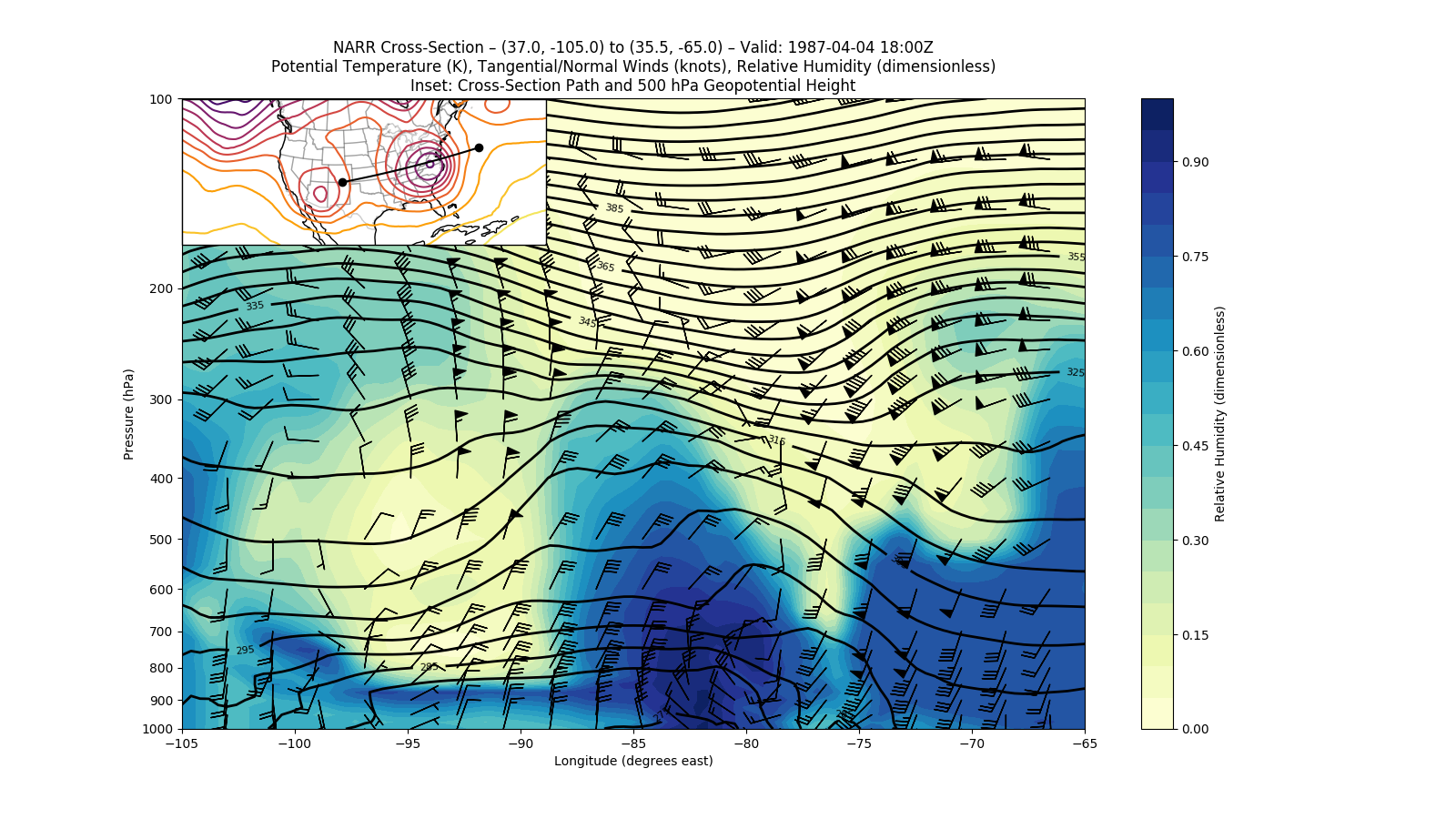
For this example, we will be plotting potential temperature, relative humidity, and tangential/normal winds. And so, we need to calculate those, and add them to the dataset:
temperature, pressure, specific_humidity = xr.broadcast(cross['Temperature'],
                                                        cross['isobaric'],
                                                        cross['Specific_humidity'])

theta = mpcalc.potential_temperature(pressure, temperature)
rh = mpcalc.relative_humidity_from_specific_humidity(specific_humidity, temperature, pressure)

# These calculations return unit arrays, so put those back into DataArrays in our Dataset
cross['Potential_temperature'] = xr.DataArray(theta,
                                              coords=temperature.coords,
                                              dims=temperature.dims,
                                              attrs={'units': theta.units})
cross['Relative_humidity'] = xr.DataArray(rh,
                                          coords=specific_humidity.coords,
                                          dims=specific_humidity.dims,
                                          attrs={'units': rh.units})

cross['u_wind'].metpy.convert_units('knots')
cross['v_wind'].metpy.convert_units('knots')
cross['t_wind'], cross['n_wind'] = mpcalc.cross_section_components(cross['u_wind'],
                                                                   cross['v_wind'])

print(cross)
Out:
<xarray.Dataset>
Dimensions:                (index: 100, isobaric: 29)
Coordinates:
    time                   datetime64[ns] 1987-04-04T18:00:00
  * isobaric               (isobaric) float64 1e+03 975.0 950.0 ... 125.0 100.0
    crs                    object Projection: lambert_conformal_conic
    x                      (index) float64 1.818e+05 2.18e+05 ... 3.712e+06
    y                      (index) float64 -1.454e+06 -1.447e+06 ... -5.573e+05
  * index                  (index) int64 0 1 2 3 4 5 6 ... 93 94 95 96 97 98 99
    lat                    (index) float64 37.0 37.05 37.11 ... 35.66 35.58 35.5
    lon                    (index) float64 -105.0 -104.6 -104.2 ... -65.39 -65.0
Data variables:
    Temperature            (isobaric, index) float64 287.7 286.9 ... 211.4 211.4
    Lambert_Conformal      |S1 ...
    u_wind                 (isobaric, index) float64 -5.304 0.9285 ... 46.03
    v_wind                 (isobaric, index) float64 16.47 11.13 ... -2.104
    Geopotential_height    (isobaric, index) float64 118.6 127.4 ... 1.636e+04
    Specific_humidity      (isobaric, index) float64 0.006367 ... 4.223e-06
    Potential_temperature  (isobaric, index) float64 287.7 286.9 ... 408.1 408.1
    Relative_humidity      (isobaric, index) float64 0.6114 0.6195 ... 0.04498
    t_wind                 (isobaric, index) float64 -2.027 3.07 ... 45.18 43.27
    n_wind                 (isobaric, index) float64 17.18 10.73 ... -15.83
Now, we can make the plot.
# Define the figure object and primary axes
fig = plt.figure(1, figsize=(16., 9.))
ax = plt.axes()

# Plot RH using contourf
rh_contour = ax.contourf(cross['lon'], cross['isobaric'], cross['Relative_humidity'],
                         levels=np.arange(0, 1.05, .05), cmap='YlGnBu')
rh_colorbar = fig.colorbar(rh_contour)

# Plot potential temperature using contour, with some custom labeling
theta_contour = ax.contour(cross['lon'], cross['isobaric'], cross['Potential_temperature'],
                           levels=np.arange(250, 450, 5), colors='k', linewidths=2)
theta_contour.clabel(theta_contour.levels[1::2], fontsize=8, colors='k', inline=1,
                     inline_spacing=8, fmt='%i', rightside_up=True, use_clabeltext=True)

# Plot winds using the axes interface directly, with some custom indexing to make the barbs
# less crowded
wind_slc_vert = list(range(0, 19, 2)) + list(range(19, 29))
wind_slc_horz = slice(5, 100, 5)
ax.barbs(cross['lon'][wind_slc_horz], cross['isobaric'][wind_slc_vert],
         cross['t_wind'][wind_slc_vert, wind_slc_horz],
         cross['n_wind'][wind_slc_vert, wind_slc_horz], color='k')

# Adjust the y-axis to be logarithmic
ax.set_yscale('symlog')
ax.set_yticklabels(np.arange(1000, 50, -100))
ax.set_ylim(cross['isobaric'].max(), cross['isobaric'].min())
ax.set_yticks(np.arange(1000, 50, -100))

# Define the CRS and inset axes
data_crs = data['Geopotential_height'].metpy.cartopy_crs
ax_inset = fig.add_axes([0.125, 0.665, 0.25, 0.25], projection=data_crs)

# Plot geopotential height at 500 hPa using xarray's contour wrapper
ax_inset.contour(data['x'], data['y'], data['Geopotential_height'].sel(isobaric=500.),
                 levels=np.arange(5100, 6000, 60), cmap='inferno')

# Plot the path of the cross section
endpoints = data_crs.transform_points(ccrs.Geodetic(),
                                      *np.vstack([start, end]).transpose()[::-1])
ax_inset.scatter(endpoints[:, 0], endpoints[:, 1], c='k', zorder=2)
ax_inset.plot(cross['x'], cross['y'], c='k', zorder=2)

# Add geographic features
ax_inset.coastlines()
ax_inset.add_feature(cfeature.STATES.with_scale('50m'), edgecolor='k', alpha=0.2, zorder=0)

# Set the titles and axes labels
ax_inset.set_title('')
ax.set_title('NARR Cross-Section \u2013 {} to {} \u2013 Valid: {}\n'
             'Potential Temperature (K), Tangential/Normal Winds (knots), '
             'Relative Humidity (dimensionless)\n'
             'Inset: Cross-Section Path and 500 hPa Geopotential Height'.format(
                 start, end, cross['time'].dt.strftime('%Y-%m-%d %H:%MZ').item()))
ax.set_ylabel('Pressure (hPa)')
ax.set_xlabel('Longitude (degrees east)')
rh_colorbar.set_label('Relative Humidity (dimensionless)')

plt.show()
Total running time of the script: ( 0 minutes 0.767 seconds)