Note
Click here to download the full example code
xarray is a powerful Python package that provides N-dimensional labeled arrays and datasets following the Common Data Model. MetPy’s suite of meteorological calculations are designed to integrate with xarray DataArrays as one of its two primary data models (the other being Pint Quantities). MetPy also provides DataArray and Dataset accessors (collections of methods and properties attached to the .metpy property) for coordinate/CRS and unit operations.
.metpy
Full information on MetPy’s accessors is available in the appropriate section of the reference guide, otherwise, continue on in this tutorial for a demonstration of the three main components of MetPy’s integration with xarray (coordinates/coordinate reference systems, units, and calculations), as well as instructive examples for both CF-compliant and non-compliant datasets.
First, some general imports…
import numpy as np import xarray as xr # Any import of metpy will activate the accessors import metpy.calc as mpcalc from metpy.cbook import get_test_data from metpy.units import units
…and opening some sample data to work with.
# Open the netCDF file as a xarray Dataset data = xr.open_dataset(get_test_data('irma_gfs_example.nc', False)) # View a summary of the Dataset data
<xarray.Dataset> Dimensions: (isobaric1: 21, isobaric3: 31, latitude: 81, longitude: 131, time1: 9) Coordinates: * time1 (time1) datetime64[ns] 2017-09-05T12... reftime datetime64[ns] 2017-09-05T12:00:00 * latitude (latitude) float32 50.0 49.5 ... 10.0 * isobaric3 (isobaric3) float64 100.0 ... 1e+05 * isobaric1 (isobaric1) float64 1e+04 ... 1e+05 * longitude (longitude) float32 250.0 ... 315.0 Data variables: Vertical_velocity_pressure_isobaric (time1, isobaric1, latitude, longitude) float32 ... Relative_humidity_isobaric (time1, isobaric3, latitude, longitude) float32 ... Temperature_isobaric (time1, isobaric3, latitude, longitude) float32 ... u-component_of_wind_isobaric (time1, isobaric3, latitude, longitude) float32 ... v-component_of_wind_isobaric (time1, isobaric3, latitude, longitude) float32 ... Geopotential_height_isobaric (time1, isobaric3, latitude, longitude) float32 ... LatLon_361X720-0p25S-180p00E int32 -2147483647 Attributes: Originating_or_generating_Center: ... Originating_or_generating_Subcenter: ... GRIB_table_version: ... Type_of_generating_process: ... Analysis_or_forecast_generating_process_identifier_defined_by_originating... Conventions: ... history: ... featureType: ... History: ... geospatial_lat_min: ... geospatial_lat_max: ... geospatial_lon_min: ... geospatial_lon_max: ...
array(['2017-09-05T12:00:00.000000000', '2017-09-05T15:00:00.000000000', '2017-09-05T18:00:00.000000000', '2017-09-05T21:00:00.000000000', '2017-09-06T00:00:00.000000000', '2017-09-06T03:00:00.000000000', '2017-09-06T06:00:00.000000000', '2017-09-06T09:00:00.000000000', '2017-09-06T12:00:00.000000000'], dtype='datetime64[ns]')
array('2017-09-05T12:00:00.000000000', dtype='datetime64[ns]')
array([50. , 49.5, 49. , 48.5, 48. , 47.5, 47. , 46.5, 46. , 45.5, 45. , 44.5, 44. , 43.5, 43. , 42.5, 42. , 41.5, 41. , 40.5, 40. , 39.5, 39. , 38.5, 38. , 37.5, 37. , 36.5, 36. , 35.5, 35. , 34.5, 34. , 33.5, 33. , 32.5, 32. , 31.5, 31. , 30.5, 30. , 29.5, 29. , 28.5, 28. , 27.5, 27. , 26.5, 26. , 25.5, 25. , 24.5, 24. , 23.5, 23. , 22.5, 22. , 21.5, 21. , 20.5, 20. , 19.5, 19. , 18.5, 18. , 17.5, 17. , 16.5, 16. , 15.5, 15. , 14.5, 14. , 13.5, 13. , 12.5, 12. , 11.5, 11. , 10.5, 10. ], dtype=float32)
array([ 100., 200., 300., 500., 700., 1000., 2000., 3000., 5000., 7000., 10000., 15000., 20000., 25000., 30000., 35000., 40000., 45000., 50000., 55000., 60000., 65000., 70000., 75000., 80000., 85000., 90000., 92500., 95000., 97500., 100000.])
array([ 10000., 15000., 20000., 25000., 30000., 35000., 40000., 45000., 50000., 55000., 60000., 65000., 70000., 75000., 80000., 85000., 90000., 92500., 95000., 97500., 100000.])
array([250. , 250.5, 251. , 251.5, 252. , 252.5, 253. , 253.5, 254. , 254.5, 255. , 255.5, 256. , 256.5, 257. , 257.5, 258. , 258.5, 259. , 259.5, 260. , 260.5, 261. , 261.5, 262. , 262.5, 263. , 263.5, 264. , 264.5, 265. , 265.5, 266. , 266.5, 267. , 267.5, 268. , 268.5, 269. , 269.5, 270. , 270.5, 271. , 271.5, 272. , 272.5, 273. , 273.5, 274. , 274.5, 275. , 275.5, 276. , 276.5, 277. , 277.5, 278. , 278.5, 279. , 279.5, 280. , 280.5, 281. , 281.5, 282. , 282.5, 283. , 283.5, 284. , 284.5, 285. , 285.5, 286. , 286.5, 287. , 287.5, 288. , 288.5, 289. , 289.5, 290. , 290.5, 291. , 291.5, 292. , 292.5, 293. , 293.5, 294. , 294.5, 295. , 295.5, 296. , 296.5, 297. , 297.5, 298. , 298.5, 299. , 299.5, 300. , 300.5, 301. , 301.5, 302. , 302.5, 303. , 303.5, 304. , 304.5, 305. , 305.5, 306. , 306.5, 307. , 307.5, 308. , 308.5, 309. , 309.5, 310. , 310.5, 311. , 311.5, 312. , 312.5, 313. , 313.5, 314. , 314.5, 315. ], dtype=float32)
[2005479 values with dtype=float32]
[2960469 values with dtype=float32]
array(-2147483647, dtype=int32)
While xarray can handle a wide variety of n-dimensional data (essentially anything that can be stored in a netCDF file), a common use case is working with gridded model output. Such model data can be obtained from a THREDDS Data Server using the siphon package, but here we’ve used an example subset of GFS data from Hurrican Irma (September 5th, 2017) included in MetPy’s test suite. Generally, a local file (or remote file via OPeNDAP) can be opened with xr.open_dataset("path").
xr.open_dataset("path")
Going back to the above object, this Dataset consists of dimensions and their associated coordinates, which in turn make up the axes along which the data variables are defined. The dataset also has a dictionary-like collection of attributes. What happens if we look at just a single data variable?
Dataset
temperature = data['Temperature_isobaric'] temperature
<xarray.DataArray 'Temperature_isobaric' (time1: 9, isobaric3: 31, latitude: 81, longitude: 131)> [2960469 values with dtype=float32] Coordinates: * time1 (time1) datetime64[ns] 2017-09-05T12:00:00 ... 2017-09-06T12:0... reftime datetime64[ns] 2017-09-05T12:00:00 * latitude (latitude) float32 50.0 49.5 49.0 48.5 ... 11.5 11.0 10.5 10.0 * isobaric3 (isobaric3) float64 100.0 200.0 300.0 ... 9.5e+04 9.75e+04 1e+05 * longitude (longitude) float32 250.0 250.5 251.0 251.5 ... 314.0 314.5 315.0 Attributes: long_name: Temperature @ Isobaric surface units: K Grib_Variable_Id: VAR_0-0-0_L100 Grib2_Parameter: [0 0 0] Grib2_Parameter_Discipline: Meteorological products Grib2_Parameter_Category: Temperature Grib2_Parameter_Name: Temperature Grib2_Level_Type: 100 Grib2_Level_Desc: Isobaric surface Grib2_Generating_Process_Type: Forecast grid_mapping: LatLon_361X720-0p25S-180p00E
This is a DataArray, which stores just a single data variable with its associated coordinates and attributes. These individual DataArrays are the kinds of objects that MetPy’s calculations take as input (more on that in Calculations section below).
DataArray
If you are more interested in learning about xarray’s terminology and data structures, see the terminology section of xarray’s documenation.
MetPy’s first set of helpers comes with identifying coordinate types. In a given dataset, coordinates can have a variety of different names and yet refer to the same type (such as “isobaric1” and “isobaric3” both referring to vertical isobaric coordinates). Following CF conventions, as well as using some fall-back regular expressions, MetPy can systematically identify coordinates of the following types:
time
vertical
latitude
y
longitude
x
When identifying a single coordinate, it is best to use the property directly associated with that type
temperature.metpy.time
<xarray.DataArray 'time1' (time1: 9)> array(['2017-09-05T12:00:00.000000000', '2017-09-05T15:00:00.000000000', '2017-09-05T18:00:00.000000000', '2017-09-05T21:00:00.000000000', '2017-09-06T00:00:00.000000000', '2017-09-06T03:00:00.000000000', '2017-09-06T06:00:00.000000000', '2017-09-06T09:00:00.000000000', '2017-09-06T12:00:00.000000000'], dtype='datetime64[ns]') Coordinates: * time1 (time1) datetime64[ns] 2017-09-05T12:00:00 ... 2017-09-06T12:00:00 reftime datetime64[ns] 2017-09-05T12:00:00 Attributes: standard_name: time long_name: time udunits: Hour since 2017-09-05T12:00:00Z _metpy_axis: time
When accessing multiple coordinate types simultaneously, you can use the .coordinates() method to yield a generator for the respective coordinates
.coordinates()
x, y = temperature.metpy.coordinates('x', 'y')
These coordinate type aliases can also be used in MetPy’s wrapped .sel and .loc for indexing and selecting on DataArrays. For example, to access 500 hPa heights at 1800Z,
.sel
.loc
heights = data['Geopotential_height_isobaric'].metpy.sel( time='2017-09-05 18:00', vertical=50000. )
(Notice how we specified 50000 here without units…we’ll go over a better alternative in the next section on units.)
One point of warning: xarray’s selection and indexing only works if these coordinates are dimension coordinates, meaning that they are 1D and share the name of their associated dimension. In practice, this means that you can’t index a dataset that has 2D latitude and longitude coordinates by latitudes and longitudes, instead, you must index by the 1D y and x dimension coordinates. (What if these coordinates are missing, you may ask? See the final subsection on .assign_y_x for more details.)
.assign_y_x
Beyond just the coordinates themselves, a common need for both calculations with and plots of geospatial data is knowing the coordinate reference system (CRS) on which the horizontal spatial coordinates are defined. MetPy follows the CF Conventions for its CRS definitions, which it then caches on the metpy_crs coordinate in order for it to persist through calculations and other array operations. There are two ways to do so in MetPy:
metpy_crs
First, if your dataset is already conforming to the CF Conventions, it will have a grid mapping variable that is associated with the other data variables by the grid_mapping attribute. This is automatically parsed via the .parse_cf() method:
grid_mapping
.parse_cf()
# Parse full dataset data_parsed = data.metpy.parse_cf() # Parse subset of dataset data_subset = data.metpy.parse_cf([ 'u-component_of_wind_isobaric', 'v-component_of_wind_isobaric', 'Vertical_velocity_pressure_isobaric' ]) # Parse single variable relative_humidity = data.metpy.parse_cf('Relative_humidity_isobaric')
If your dataset doesn’t have a CF-conforming grid mapping variable, you can manually specify the CRS using the .assign_crs() method:
.assign_crs()
temperature = data['Temperature_isobaric'].metpy.assign_crs( grid_mapping_name='latitude_longitude', earth_radius=6371229.0 ) temperature
<xarray.DataArray 'Temperature_isobaric' (time1: 9, isobaric3: 31, latitude: 81, longitude: 131)> [2960469 values with dtype=float32] Coordinates: * time1 (time1) datetime64[ns] 2017-09-05T12:00:00 ... 2017-09-06T12:0... reftime datetime64[ns] 2017-09-05T12:00:00 * latitude (latitude) float32 50.0 49.5 49.0 48.5 ... 11.5 11.0 10.5 10.0 * isobaric3 (isobaric3) float64 100.0 200.0 300.0 ... 9.5e+04 9.75e+04 1e+05 * longitude (longitude) float32 250.0 250.5 251.0 251.5 ... 314.0 314.5 315.0 metpy_crs object Projection: latitude_longitude Attributes: long_name: Temperature @ Isobaric surface units: K Grib_Variable_Id: VAR_0-0-0_L100 Grib2_Parameter: [0 0 0] Grib2_Parameter_Discipline: Meteorological products Grib2_Parameter_Category: Temperature Grib2_Parameter_Name: Temperature Grib2_Level_Type: 100 Grib2_Level_Desc: Isobaric surface Grib2_Generating_Process_Type: Forecast grid_mapping: LatLon_361X720-0p25S-180p00E
array(<metpy.plots.mapping.CFProjection object at 0x7f98bd028430>, dtype=object)
Notice the newly added metpy_crs non-dimension coordinate. Now how can we use this in practice? For individual DataArrayss, we can access the cartopy and pyproj objects corresponding to this CRS:
DataArrays
# Cartopy CRS, useful for plotting relative_humidity.metpy.cartopy_crs
<cartopy.crs.PlateCarree object at 0x7f98bd117b80>
# pyproj CRS, useful for projection transformations and forward/backward azimuth and great # circle calculations temperature.metpy.pyproj_crs
Out:
<Geographic 2D CRS: {"$schema": "https://proj.org/schemas/v0.2/projjso ...> Name: undefined Axis Info [ellipsoidal]: - lon[east]: Longitude (degree) - lat[north]: Latitude (degree) Area of Use: - undefined Datum: undefined - Ellipsoid: undefined - Prime Meridian: Greenwich
Finally, there are times when a certain horizontal coordinate type is missing from your dataset, and you need the other, that is, you have latitude/longitude and need y/x, or visa versa. This is where the .assign_y_x and .assign_latitude_longitude methods come in handy. Our current GFS sample won’t work to demonstrate this (since, on its latitude-longitude grid, y is latitude and x is longitude), so for more information, take a look at the Non-Compliant Dataset Example below, or view the accessor documentation.
.assign_latitude_longitude
Since unit-aware calculations are a major part of the MetPy library, unit support is a major part of MetPy’s xarray integration!
One very important point of consideration is that xarray data variables (in both Datasets and DataArrays) can store both unit-aware and unit-naive array types. Unit-naive array types will be used by default in xarray, so we need to convert to a unit-aware type if we want to use xarray operations while preserving unit correctness. MetPy provides the .quantify() method for this (named since we are turning the data stored inside the xarray object into a Pint Quantity object)
.quantify()
Quantity
heights = heights.metpy.quantify() heights
<xarray.DataArray 'Geopotential_height_isobaric' (latitude: 81, longitude: 131)> <Quantity([[5883.3564 5879.3164 5875.3564 ... 5769.3965 5769.996 5770.436 ] [5885.476 5882.2363 5877.6763 ... 5783.916 5784.516 5785.1963] [5888.8765 5885.1562 5880.916 ... 5798.476 5799.076 5799.7163] ... [5892.516 5892.2363 5891.996 ... 5881.556 5881.436 5880.596 ] [5891.8364 5891.596 5891.7163 ... 5880.2764 5880.3564 5879.916 ] [5891.3564 5891.596 5891.3564 ... 5879.8765 5879.596 5878.996 ]], 'meter')> Coordinates: time1 datetime64[ns] 2017-09-05T18:00:00 reftime datetime64[ns] 2017-09-05T12:00:00 * latitude (latitude) float32 50.0 49.5 49.0 48.5 ... 11.5 11.0 10.5 10.0 isobaric3 float64 5e+04 * longitude (longitude) float32 250.0 250.5 251.0 251.5 ... 314.0 314.5 315.0 Attributes: long_name: Geopotential height @ Isobaric surface Grib_Variable_Id: VAR_0-3-5_L100 Grib2_Parameter: [0 3 5] Grib2_Parameter_Discipline: Meteorological products Grib2_Parameter_Category: Mass Grib2_Parameter_Name: Geopotential height Grib2_Level_Type: 100 Grib2_Level_Desc: Isobaric surface Grib2_Generating_Process_Type: Forecast grid_mapping: LatLon_361X720-0p25S-180p00E
[[5883.3564453125 5879.31640625 5875.3564453125 ... 5769.396484375 5769.99609375 5770.43603515625] [5885.47607421875 5882.236328125 5877.67626953125 ... 5783.916015625 5784.51611328125 5785.1962890625] [5888.87646484375 5885.15625 5880.916015625 ... 5798.47607421875 5799.076171875 5799.71630859375] ... [5892.51611328125 5892.236328125 5891.99609375 ... 5881.55615234375 5881.43603515625 5880.59619140625] [5891.83642578125 5891.59619140625 5891.71630859375 ... 5880.2763671875 5880.3564453125 5879.916015625] [5891.3564453125 5891.59619140625 5891.3564453125 ... 5879.87646484375 5879.59619140625 5878.99609375]]
array('2017-09-05T18:00:00.000000000', dtype='datetime64[ns]')
array(50000.)
Notice how the units are now represented in the data itself, rather than as a text attribute. Now, even if we perform some kind of xarray operation (such as taking the zonal mean), the units are preserved
heights_mean = heights.mean('longitude') heights_mean
<xarray.DataArray 'Geopotential_height_isobaric' (latitude: 81)> <Quantity([5636.367 5644.392 5652.7705 5661.369 5669.813 5678.5083 5687.433 5696.517 5705.927 5715.6123 5725.702 5736.1387 5746.884 5757.718 5768.566 5779.2812 5789.8193 5799.801 5809.502 5818.7715 5827.7744 5836.921 5846.3857 5855.668 5864.2397 5871.804 5878.769 5885.058 5890.129 5894.0293 5897.146 5899.633 5901.674 5903.2773 5904.41 5905.27 5905.897 5906.592 5907.0083 5907.0806 5907.031 5906.871 5906.777 5906.4556 5906.121 5905.798 5905.6826 5905.5986 5905.4097 5905.1245 5904.773 5904.43 5903.954 5903.378 5902.532 5901.714 5900.865 5900.0933 5899.336 5898.4673 5897.44 5896.233 5895.057 5893.633 5891.532 5888.15 5883.094 5884.8022 5887.923 5889.0054 5889.114 5888.8887 5888.685 5888.146 5887.567 5887.0317 5886.299 5885.4214 5884.515 5883.694 5883.072 ], 'meter')> Coordinates: time1 datetime64[ns] 2017-09-05T18:00:00 reftime datetime64[ns] 2017-09-05T12:00:00 * latitude (latitude) float32 50.0 49.5 49.0 48.5 ... 11.5 11.0 10.5 10.0 isobaric3 float64 5e+04
[5636.3671875 5644.39208984375 5652.7705078125 5661.369140625 5669.81298828125 5678.50830078125 5687.43310546875 5696.51708984375 5705.9267578125 5715.6123046875 5725.7021484375 5736.138671875 5746.8837890625 5757.7177734375 5768.56591796875 5779.28125 5789.8193359375 5799.80078125 5809.501953125 5818.771484375 5827.7744140625 5836.9208984375 5846.3857421875 5855.66796875 5864.23974609375 5871.80419921875 5878.76904296875 5885.05810546875 5890.12890625 5894.029296875 5897.14599609375 5899.6328125 5901.673828125 5903.27734375 5904.41015625 5905.27001953125 5905.89697265625 5906.591796875 5907.00830078125 5907.08056640625 5907.03076171875 5906.87109375 5906.77685546875 5906.45556640625 5906.12109375 5905.7978515625 5905.6826171875 5905.5986328125 5905.40966796875 5905.12451171875 5904.77294921875 5904.43017578125 5903.9541015625 5903.3779296875 5902.5322265625 5901.7138671875 5900.865234375 5900.09326171875 5899.3359375 5898.46728515625 5897.43994140625 5896.23291015625 5895.05712890625 5893.6328125 5891.5322265625 5888.14990234375 5883.09423828125 5884.80224609375 5887.9228515625 5889.00537109375 5889.11376953125 5888.888671875 5888.68505859375 5888.14599609375 5887.56689453125 5887.03173828125 5886.298828125 5885.42138671875 5884.51513671875 5883.69384765625 5883.07177734375]
However, this “quantification” is not without its consequences. By default, xarray loads its data lazily to conserve memory usage. Unless your data is chunked into a Dask array (using the chunks argument), this .quantify() method will load data into memory, which could slow your script or even cause your process to run out of memory. And so, we recommend subsetting your data before quantifying it.
chunks
Also, these Pint Quantity data objects are not properly handled by xarray when writing to disk. And so, if you want to safely export your data, you will need to undo the quantification with the .dequantify() method, which converts your data back to a unit-naive array with the unit as a text attribute
.dequantify()
heights_mean_str_units = heights_mean.metpy.dequantify() heights_mean_str_units
<xarray.DataArray 'Geopotential_height_isobaric' (latitude: 81)> array([5636.367 , 5644.392 , 5652.7705, 5661.369 , 5669.813 , 5678.5083, 5687.433 , 5696.517 , 5705.927 , 5715.6123, 5725.702 , 5736.1387, 5746.884 , 5757.718 , 5768.566 , 5779.2812, 5789.8193, 5799.801 , 5809.502 , 5818.7715, 5827.7744, 5836.921 , 5846.3857, 5855.668 , 5864.2397, 5871.804 , 5878.769 , 5885.058 , 5890.129 , 5894.0293, 5897.146 , 5899.633 , 5901.674 , 5903.2773, 5904.41 , 5905.27 , 5905.897 , 5906.592 , 5907.0083, 5907.0806, 5907.031 , 5906.871 , 5906.777 , 5906.4556, 5906.121 , 5905.798 , 5905.6826, 5905.5986, 5905.4097, 5905.1245, 5904.773 , 5904.43 , 5903.954 , 5903.378 , 5902.532 , 5901.714 , 5900.865 , 5900.0933, 5899.336 , 5898.4673, 5897.44 , 5896.233 , 5895.057 , 5893.633 , 5891.532 , 5888.15 , 5883.094 , 5884.8022, 5887.923 , 5889.0054, 5889.114 , 5888.8887, 5888.685 , 5888.146 , 5887.567 , 5887.0317, 5886.299 , 5885.4214, 5884.515 , 5883.694 , 5883.072 ], dtype=float32) Coordinates: time1 datetime64[ns] 2017-09-05T18:00:00 reftime datetime64[ns] 2017-09-05T12:00:00 * latitude (latitude) float32 50.0 49.5 49.0 48.5 ... 11.5 11.0 10.5 10.0 isobaric3 float64 5e+04 Attributes: units: meter
array([5636.367 , 5644.392 , 5652.7705, 5661.369 , 5669.813 , 5678.5083, 5687.433 , 5696.517 , 5705.927 , 5715.6123, 5725.702 , 5736.1387, 5746.884 , 5757.718 , 5768.566 , 5779.2812, 5789.8193, 5799.801 , 5809.502 , 5818.7715, 5827.7744, 5836.921 , 5846.3857, 5855.668 , 5864.2397, 5871.804 , 5878.769 , 5885.058 , 5890.129 , 5894.0293, 5897.146 , 5899.633 , 5901.674 , 5903.2773, 5904.41 , 5905.27 , 5905.897 , 5906.592 , 5907.0083, 5907.0806, 5907.031 , 5906.871 , 5906.777 , 5906.4556, 5906.121 , 5905.798 , 5905.6826, 5905.5986, 5905.4097, 5905.1245, 5904.773 , 5904.43 , 5903.954 , 5903.378 , 5902.532 , 5901.714 , 5900.865 , 5900.0933, 5899.336 , 5898.4673, 5897.44 , 5896.233 , 5895.057 , 5893.633 , 5891.532 , 5888.15 , 5883.094 , 5884.8022, 5887.923 , 5889.0054, 5889.114 , 5888.8887, 5888.685 , 5888.146 , 5887.567 , 5887.0317, 5886.299 , 5885.4214, 5884.515 , 5883.694 , 5883.072 ], dtype=float32)
Other useful unit integration features include:
Unit-based selection/indexing:
heights_at_45_north = data['Geopotential_height_isobaric'].metpy.sel( latitude=45 * units.degrees_north, vertical=300 * units.hPa ) heights_at_45_north
<xarray.DataArray 'Geopotential_height_isobaric' (time1: 9, longitude: 131)> array([[9682.115, 9676.315, 9673.275, ..., 9608.755, 9609.035, 9609.395], [9683.031, 9678.352, 9675.312, ..., 9623.551, 9624.352, 9625.071], [9688.037, 9685.677, 9681.677, ..., 9631.757, 9632.437, 9633.157], ..., [9677.054, 9678.254, 9669.454, ..., 9656.294, 9656.054, 9655.894], [9665.767, 9666.247, 9658.087, ..., 9666.047, 9665.487, 9664.887], [9660.616, 9659.856, 9652.017, ..., 9681.176, 9680.097, 9679.097]], dtype=float32) Coordinates: * time1 (time1) datetime64[ns] 2017-09-05T12:00:00 ... 2017-09-06T12:0... reftime datetime64[ns] 2017-09-05T12:00:00 latitude float32 45.0 isobaric3 float64 3e+04 * longitude (longitude) float32 250.0 250.5 251.0 251.5 ... 314.0 314.5 315.0 Attributes: long_name: Geopotential height @ Isobaric surface units: gpm Grib_Variable_Id: VAR_0-3-5_L100 Grib2_Parameter: [0 3 5] Grib2_Parameter_Discipline: Meteorological products Grib2_Parameter_Category: Mass Grib2_Parameter_Name: Geopotential height Grib2_Level_Type: 100 Grib2_Level_Desc: Isobaric surface Grib2_Generating_Process_Type: Forecast grid_mapping: LatLon_361X720-0p25S-180p00E
array([[9682.115, 9676.315, 9673.275, ..., 9608.755, 9609.035, 9609.395], [9683.031, 9678.352, 9675.312, ..., 9623.551, 9624.352, 9625.071], [9688.037, 9685.677, 9681.677, ..., 9631.757, 9632.437, 9633.157], ..., [9677.054, 9678.254, 9669.454, ..., 9656.294, 9656.054, 9655.894], [9665.767, 9666.247, 9658.087, ..., 9666.047, 9665.487, 9664.887], [9660.616, 9659.856, 9652.017, ..., 9681.176, 9680.097, 9679.097]], dtype=float32)
array(45., dtype=float32)
array(30000.)
Unit conversion:
temperature_degC = temperature[0].metpy.convert_units('degC') temperature_degC
<xarray.DataArray 'Temperature_isobaric' (isobaric3: 31, latitude: 81, longitude: 131)> <Quantity([[[-15.149994 -15.149994 -15.25 ... -14.949982 -14.949982 -14.850006] [-15.25 -15.25 -15.350006 ... -14.949982 -14.949982 -14.949982] [-15.350006 -15.350006 -15.350006 ... -15.049988 -15.049988 -15.049988] ... [-12.350006 -12.350006 -12.350006 ... -15.149994 -15.049988 -14.949982] [-12.149994 -12.149994 -12.149994 ... -15.049988 -15.049988 -14.949982] [-11.949982 -11.949982 -11.949982 ... -15.049988 -14.949982 -14.850006]] [[-16.649994 -16.649994 -16.649994 ... -17.549988 -17.549988 -17.649994] [-16.75 -16.75 -16.850006 ... -17.649994 -17.649994 -17.649994] [-16.949982 -16.949982 -16.949982 ... -17.75 -17.75 -17.75 ] ... [-14.049988 -14.049988 -14.049988 ... -12.049988 -11.75 -11.549988] [-13.949982 -13.949982 -13.949982 ... -12.049988 -11.75 -11.549988] [-13.75 -13.850006 -13.850006 ... -12.049988 -11.75 -11.549988]] [[-21.75 -21.75 -21.75 ... -22.649994 -22.649994 -22.649994] [-21.949997 -21.84999 -21.84999 ... -22.75 -22.75 -22.75 ] [-22.049988 -22.049988 -22.049988 ... -22.84999 -22.84999 -22.949997] ... ... ... [ 22.149994 22.149994 22.149994 ... 22.550018 22.649994 22.75 ] [ 22.050018 22.050018 21.950012 ... 22.550018 22.149994 22.350006] [ 21.950012 21.75 22.149994 ... 22.550018 22.450012 22.050018]] [[ 15.649994 15.149994 14.649994 ... 11.950012 11.850006 11.75 ] [ 15.149994 15.149994 15.050018 ... 11.950012 11.649994 11.450012] [ 15.050018 14.850006 15.050018 ... 11.850006 11.75 11.649994] ... [ 24.149994 24.25 24.149994 ... 24.649994 24.649994 24.850006] [ 23.950012 23.950012 23.850006 ... 24.649994 24.25 24.450012] [ 23.850006 23.649994 23.75 ... 24.649994 24.25 24.050018]] [[ 17.050018 16.550018 16.050018 ... 13.450012 13.450012 13.550018] [ 16.550018 16.550018 16.450012 ... 13.350006 13.050018 12.950012] [ 16.450012 16.25 16.450012 ... 13.050018 12.850006 12.850006] ... [ 26.350006 26.350006 26.25 ... 26.75 26.850006 26.950012] [ 26.050018 26.050018 25.950012 ... 26.75 26.350006 26.550018] [ 26.050018 25.75 25.649994 ... 26.75 26.350006 26.149994]]], 'degree_Celsius')> Coordinates: time1 datetime64[ns] 2017-09-05T12:00:00 reftime datetime64[ns] 2017-09-05T12:00:00 * latitude (latitude) float32 50.0 49.5 49.0 48.5 ... 11.5 11.0 10.5 10.0 * isobaric3 (isobaric3) float64 100.0 200.0 300.0 ... 9.5e+04 9.75e+04 1e+05 * longitude (longitude) float32 250.0 250.5 251.0 251.5 ... 314.0 314.5 315.0 metpy_crs object Projection: latitude_longitude Attributes: long_name: Temperature @ Isobaric surface Grib_Variable_Id: VAR_0-0-0_L100 Grib2_Parameter: [0 0 0] Grib2_Parameter_Discipline: Meteorological products Grib2_Parameter_Category: Temperature Grib2_Parameter_Name: Temperature Grib2_Level_Type: 100 Grib2_Level_Desc: Isobaric surface Grib2_Generating_Process_Type: Forecast grid_mapping: LatLon_361X720-0p25S-180p00E
[[[-15.149993896484375 -15.149993896484375 -15.25 ... -14.949981689453125 -14.949981689453125 -14.850006103515625] [-15.25 -15.25 -15.350006103515625 ... -14.949981689453125 -14.949981689453125 -14.949981689453125] [-15.350006103515625 -15.350006103515625 -15.350006103515625 ... -15.04998779296875 -15.04998779296875 -15.04998779296875] ... [-12.350006103515625 -12.350006103515625 -12.350006103515625 ... -15.149993896484375 -15.04998779296875 -14.949981689453125] [-12.149993896484375 -12.149993896484375 -12.149993896484375 ... -15.04998779296875 -15.04998779296875 -14.949981689453125] [-11.949981689453125 -11.949981689453125 -11.949981689453125 ... -15.04998779296875 -14.949981689453125 -14.850006103515625]] [[-16.649993896484375 -16.649993896484375 -16.649993896484375 ... -17.54998779296875 -17.54998779296875 -17.649993896484375] [-16.75 -16.75 -16.850006103515625 ... -17.649993896484375 -17.649993896484375 -17.649993896484375] [-16.949981689453125 -16.949981689453125 -16.949981689453125 ... -17.75 -17.75 -17.75] ... [-14.04998779296875 -14.04998779296875 -14.04998779296875 ... -12.04998779296875 -11.75 -11.54998779296875] [-13.949981689453125 -13.949981689453125 -13.949981689453125 ... -12.04998779296875 -11.75 -11.54998779296875] [-13.75 -13.850006103515625 -13.850006103515625 ... -12.04998779296875 -11.75 -11.54998779296875]] [[-21.75 -21.75 -21.75 ... -22.649993896484375 -22.649993896484375 -22.649993896484375] [-21.949996948242188 -21.849990844726562 -21.849990844726562 ... -22.75 -22.75 -22.75] [-22.04998779296875 -22.04998779296875 -22.04998779296875 ... -22.849990844726562 -22.849990844726562 -22.949996948242188] ... [-22.149993896484375 -22.149993896484375 -22.149993896484375 ... -18.849990844726562 -18.949996948242188 -19.149993896484375] [-22.04998779296875 -22.04998779296875 -22.04998779296875 ... -18.349990844726562 -18.449996948242188 -18.649993896484375] [-21.949996948242188 -21.949996948242188 -21.949996948242188 ... -17.849990844726562 -18.04998779296875 -18.149993896484375]] ... [[14.25 13.75 13.149993896484375 ... 12.550018310546875 11.45001220703125 11.050018310546875] [13.75 13.75 13.649993896484375 ... 12.350006103515625 11.95001220703125 11.75] [13.649993896484375 13.45001220703125 13.649993896484375 ... 12.149993896484375 12.050018310546875 12.149993896484375] ... [22.149993896484375 22.149993896484375 22.149993896484375 ... 22.550018310546875 22.649993896484375 22.75] [22.050018310546875 22.050018310546875 21.95001220703125 ... 22.550018310546875 22.149993896484375 22.350006103515625] [21.95001220703125 21.75 22.149993896484375 ... 22.550018310546875 22.45001220703125 22.050018310546875]] [[15.649993896484375 15.149993896484375 14.649993896484375 ... 11.95001220703125 11.850006103515625 11.75] [15.149993896484375 15.149993896484375 15.050018310546875 ... 11.95001220703125 11.649993896484375 11.45001220703125] [15.050018310546875 14.850006103515625 15.050018310546875 ... 11.850006103515625 11.75 11.649993896484375] ... [24.149993896484375 24.25 24.149993896484375 ... 24.649993896484375 24.649993896484375 24.850006103515625] [23.95001220703125 23.95001220703125 23.850006103515625 ... 24.649993896484375 24.25 24.45001220703125] [23.850006103515625 23.649993896484375 23.75 ... 24.649993896484375 24.25 24.050018310546875]] [[17.050018310546875 16.550018310546875 16.050018310546875 ... 13.45001220703125 13.45001220703125 13.550018310546875] [16.550018310546875 16.550018310546875 16.45001220703125 ... 13.350006103515625 13.050018310546875 12.95001220703125] [16.45001220703125 16.25 16.45001220703125 ... 13.050018310546875 12.850006103515625 12.850006103515625] ... [26.350006103515625 26.350006103515625 26.25 ... 26.75 26.850006103515625 26.95001220703125] [26.050018310546875 26.050018310546875 25.95001220703125 ... 26.75 26.350006103515625 26.550018310546875] [26.050018310546875 25.75 25.649993896484375 ... 26.75 26.350006103515625 26.149993896484375]]]
array(<metpy.plots.mapping.CFProjection object at 0x7f98bd090490>, dtype=object)
Unit conversion for coordinates:
heights_on_hPa_levels = heights.metpy.convert_coordinate_units('isobaric3', 'hPa') heights_on_hPa_levels['isobaric3']
<xarray.DataArray 'isobaric3' ()> array(500.) Coordinates: time1 datetime64[ns] 2017-09-05T18:00:00 reftime datetime64[ns] 2017-09-05T12:00:00 isobaric3 float64 500.0 Attributes: units: hPa positive: down _metpy_axis: vertical
array(500.)
Accessing just the underlying unit array:
heights_unit_array = heights.metpy.unit_array heights_unit_array
Accessing just the underlying units:
height_units = heights.metpy.units height_units
MetPy’s xarray integration extends to its calcuation suite as well. Most grid-capable calculations (such as thermodynamics, kinematics, and smoothers) fully support xarray DataArrays by accepting them as inputs, returning them as outputs, and automatically using the attached coordinate data/metadata to determine grid arguments
heights = data_parsed.metpy.parse_cf('Geopotential_height_isobaric').metpy.sel( time='2017-09-05 18:00', vertical=500 * units.hPa ) u_g, v_g = mpcalc.geostrophic_wind(heights) u_g
<xarray.DataArray (latitude: 81, longitude: 131)> <Quantity([[ 2.33535886 4.60981877 2.93625413 ... 22.89067952 22.89183583 23.49234567] [ 4.38966801 4.64400083 4.42111986 ... 23.12487204 23.12526033 23.28446103] [ 5.54483395 4.9994661 5.35235118 ... 22.97939121 22.94731075 22.75482798] ... [-3.42134235 -3.29600145 -3.16911313 ... -7.60556204 -6.84423212 -4.56488464] [-3.84801887 -2.12410641 -2.1224862 ... -5.57355154 -6.1049832 -5.30945593] [-2.64743317 2.22914893 -2.78516091 ... 0.27885616 -4.18284239 -7.24175843]], 'meter / second')> Coordinates: time1 datetime64[ns] 2017-09-05T18:00:00 reftime datetime64[ns] 2017-09-05T12:00:00 * latitude (latitude) float32 50.0 49.5 49.0 48.5 ... 11.5 11.0 10.5 10.0 * longitude (longitude) float32 250.0 250.5 251.0 251.5 ... 314.0 314.5 315.0 metpy_crs object Projection: latitude_longitude isobaric3 float64 5e+04
[[2.3353588579406686 4.60981877223844 2.9362541310137718 ... 22.890679520432215 22.891835829490446 23.49234566620837] [4.389668010973033 4.644000832484165 4.421119856074913 ... 23.124872038344872 23.125260332728804 23.284461030163367] [5.54483394787313 4.999466098910912 5.352351177650735 ... 22.979391208366312 22.94731074666258 22.754827976440804] ... [-3.4213423527971765 -3.296001452492959 -3.1691131336642333 ... -7.605562037088769 -6.844232124116416 -4.5648846407753245] [-3.8480188676824527 -2.1241064149587885 -2.122486196488429 ... -5.573551538876476 -6.104983197236323 -5.309455928166912] [-2.647433169930482 2.2291489311550605 -2.785160907090209 ... 0.27885615921944024 -4.182842387936929 -7.2417584269395885]]
array(<metpy.plots.mapping.CFProjection object at 0x7f98bd090820>, dtype=object)
For profile-based calculations (and most remaining calculations in the metpy.calc module), xarray DataArrays are accepted as inputs, but the outputs remain Pint Quantities (typically scalars)
metpy.calc
data_at_point = data.metpy.sel( time1='2017-09-05 12:00', latitude=40 * units.degrees_north, longitude=260 * units.degrees_east ) dewpoint = mpcalc.dewpoint_from_relative_humidity( data_at_point['Temperature_isobaric'], data_at_point['Relative_humidity_isobaric'] ) cape, cin = mpcalc.surface_based_cape_cin( data_at_point['isobaric3'], data_at_point['Temperature_isobaric'], dewpoint ) cape
/opt/hostedtoolcache/Python/3.9.1/x64/lib/python3.9/site-packages/metpy/interpolate/one_dimension.py:147: UserWarning: Interpolation point out of data bounds encountered warnings.warn('Interpolation point out of data bounds encountered')
A few remaining portions of MetPy’s calculations (mainly the interpolation module and a few other functions) do not fully support xarray, and so, use of .values may be needed to convert to a bare NumPy array. For full information on xarray support for your function of interest, see the Reference Guide.
.values
The GFS sample used throughout this tutorial so far has been an example of a CF-compliant dataset. These kinds of datasets are easiest to work with it MetPy, since most of the “xarray magic” uses CF metadata. For this kind of dataset, a typical workflow looks like the following
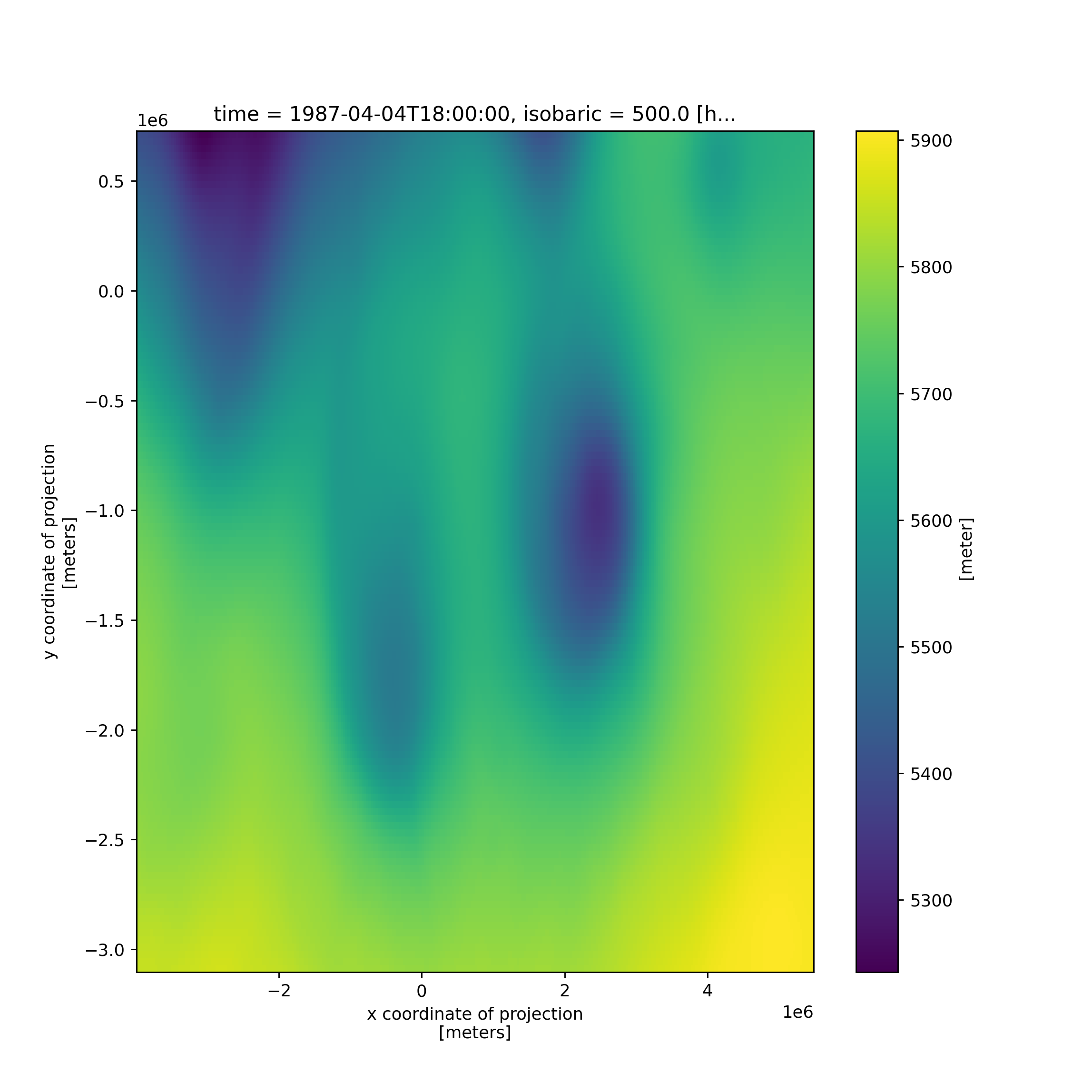
# Load data, parse it for a CF grid mapping, and promote lat/lon data variables to coordinates data = xr.open_dataset( get_test_data('narr_example.nc', False) ).metpy.parse_cf().set_coords(['lat', 'lon']) # Subset to only the data you need to save on memory usage subset = data.metpy.sel(isobaric=500 * units.hPa) # Quantify if you plan on performing xarray operations that need to maintain unit correctness subset = subset.metpy.quantify() # Perform calculations heights = mpcalc.smooth_gaussian(subset['Geopotential_height'], 5) subset['u_geo'], subset['v_geo'] = mpcalc.geostrophic_wind(heights) # Plot heights.plot()
<matplotlib.collections.QuadMesh object at 0x7f98bf5f0fa0>
# Save output subset.metpy.dequantify().drop_vars('metpy_crs').to_netcdf('500hPa_analysis.nc')
When CF metadata (such as grid mapping, coordinate attributes, etc.) are missing, a bit more work is required to manually supply the required information, for example,
nonstandard = xr.Dataset({ 'temperature': (('y', 'x'), np.arange(0, 9).reshape(3, 3) * units.degC), 'y': ('y', np.arange(0, 3) * 1e5, {'units': 'km'}), 'x': ('x', np.arange(0, 3) * 1e5, {'units': 'km'}) }) # Add both CRS and then lat/lon coords using chained methods data = nonstandard.metpy.assign_crs( grid_mapping_name='lambert_conformal_conic', latitude_of_projection_origin=38.5, longitude_of_central_meridian=262.5, standard_parallel=38.5, earth_radius=6371229.0 ).metpy.assign_latitude_longitude() # Preview the changes data
<xarray.Dataset> Dimensions: (x: 3, y: 3) Coordinates: * y (y) float64 0.0 1e+05 2e+05 * x (x) float64 0.0 1e+05 2e+05 metpy_crs object Projection: lambert_conformal_conic latitude (y, x) float64 38.5 38.49 38.48 39.4 ... 39.38 40.3 40.29 40.28 longitude (y, x) float64 -97.5 -96.35 -95.2 -97.5 ... -97.5 -96.32 -95.14 Data variables: temperature (y, x) int64 <Quantity([[0 1 2] [3 4 5] [6 7 8]], 'degree_...
array([ 0., 100000., 200000.])
array(<metpy.plots.mapping.CFProjection object at 0x7f98bf726fa0>, dtype=object)
array([[38.5 , 38.49438649, 38.47754859], [39.39925224, 39.39356847, 39.37651982], [40.29828138, 40.29252697, 40.27526648]])
array([[-97.5 , -96.35096705, -95.20229214], [-97.5 , -96.33644176, -95.17325532], [-97.5 , -96.32154456, -95.14347537]])
[[0 1 2] [3 4 5] [6 7 8]]
Once the CRS and additional coordinates are assigned, you can generally proceed as you would for a CF-compliant dataset.
Depending on your dataset and what you are trying to do, you might run into problems with xarray and MetPy. Below are examples of some of the most common issues
Multiple coordinate conflict
An axis not being available
An axis not being interpretable
UndefinedUnitError
Coordinate Conflict
Code:
x = data['Temperature'].metpy.x
Error Message:
/home/user/env/MetPy/metpy/xarray.py:305: UserWarning: More than one x coordinate present for variable "Temperature".
Fix:
Manually assign the coordinates using the assign_coordinates() method on your DataArray, or by specifying the coordinates argument to the parse_cf() method on your Dataset, to map the time, vertical, y, latitude, x, and longitude axes (as applicable to your data) to the corresponding coordinates.
assign_coordinates()
coordinates
parse_cf()
data['Temperature'].assign_coordinates({'time': 'time', 'vertical': 'isobaric', 'y': 'y', 'x': 'x'}) x = data['Temperature'].metpy.x
or
temperature = data.metpy.parse_cf('Temperature', coordinates={'time': 'time', 'vertical': 'isobaric', 'y': 'y', 'x': 'x'}) x = temperature.metpy.x
Axis Unavailable
data['Temperature'].metpy.vertical
AttributeError: vertical attribute is not available.
This means that your data variable does not have the coordinate that was requested, at least as far as the parser can recognize. Verify that you are requesting a coordinate that your data actually has, and if it still is not available, you will need to manually specify the coordinates as discussed above.
Axis Not Interpretable
x, y, ensemble = data['Temperature'].metpy.coordinates('x', 'y', 'ensemble')
AttributeError: 'ensemble' is not an interpretable axis
This means that you are requesting a coordinate that MetPy is (currently) unable to parse. While this means it cannot be recognized automatically, you can still obtain your desired coordinate directly by accessing it by name. If you have a need for systematic identification of a new coordinate type, we welcome pull requests for such new functionality on GitHub!
Undefined Unit Error
If the units attribute on your xarray data is not recognizable by Pint, you will likely recieve an UndefinedUnitError. In this case, you will likely have to update the units attribute to one that can be parsed properly by Pint. It is our aim to have all valid CF/UDUNITS unit strings be parseable, but this work is ongoing. If many variables in your dataset are not parseable, the .update_attribute method on the MetPy accessor may come in handy.
.update_attribute
Total running time of the script: ( 0 minutes 1.111 seconds)
Gallery generated by Sphinx-Gallery