Precipitation Accumulation Region of Interest¶

Python-AWIPS Tutorial Notebook

Colorized Precipation Accumulation with Identified Region of Interest

Objectives¶

Access the model data from an EDEX server and limit the data returned by using model specific parameters
Calculate the total precipitation over several model runs
Create a colorized plot for the continental US of the accumulated precipitation data
Calculate and identify area of highest of precipitation
Use higher resolution data to draw region of interest

Imports¶

The imports below are used throughout the notebook. Note the first import is coming directly from python-awips and allows us to connect to an EDEX server. The subsequent imports are for data manipulation and visualization.

from awips.dataaccess import DataAccessLayer
import cartopy.crs as ccrs
import matplotlib.pyplot as plt
from metpy.units import units
import numpy as np
from shapely.geometry import Point, Polygon

Top

Initial Setup¶

Geographic Filter¶

By defining a bounding box for the Continental US (CONUS), we’re able to optimize the data request sent to the EDEX server.

conus=[-125, -65, 25, 55]
conus_envelope = Polygon([(conus[0],conus[2]),(conus[0],conus[3]),
                          (conus[1],conus[3]),(conus[1],conus[2]),
                          (conus[0],conus[2])])

EDEX Connection¶

First we establish a connection to Unidata’s public EDEX server. With that connection made, we can create a new data request object and set the data type to grid, and use the geographic envelope we just created.

DataAccessLayer.changeEDEXHost("edex-cloud.unidata.ucar.edu")
request = DataAccessLayer.newDataRequest("grid", envelope=conus_envelope)

Refine the Request¶

Here we specify which model we’re interested in by setting the LocationNames, and the specific data we’re interested in by setting the Levels and Parameters.

request.setLocationNames("GFS1p0")
request.setLevels("0.0SFC")
request.setParameters("TP")

Get Times¶

We need to get the available times and cycles for our model data

cycles = DataAccessLayer.getAvailableTimes(request, True)
times = DataAccessLayer.getAvailableTimes(request)
fcstRun = DataAccessLayer.getForecastRun(cycles[-1], times)

Top

Function: calculate_accumulated_precip()¶

Since we’ll want to calculate the accumulated precipitation of our data more than once, it makes sense to create a function that we can call instead of duplicating the logic.

This function cycles through all the grid data responses and adds up all of the rainfall to produce a numpy array with the total ammount of rainfall for the given data request. It also finds the maximum rainfall point in x and y coordinates.

def calculate_accumulated_precip(dataRequest, forecastRun):

    for i, tt in enumerate(forecastRun):
        response = DataAccessLayer.getGridData(dataRequest, [tt])
        grid = response[0]
        if i>0:
            data += grid.getRawData()
        else:
            data = grid.getRawData()
        data[data <= -9999] = 0
        print(data.min(), data.max(), grid.getDataTime().getFcstTime()/3600)

    # Convert from mm to inches
    result = (data * units.mm).to(units.inch)
    
    ii,jj = np.where(result==result.max())
    i=ii[0]
    j=jj[0]

    return result, i, j

Top

Fuction: make_map()¶

This function creates the basics of the map we’re going to plot our data on. It takes in a bounding box to determine the extent and then adds coastlines for easy frame of reference.

def make_map(bbox, projection=ccrs.PlateCarree()):
    fig, ax = plt.subplots(figsize=(20, 14),
            subplot_kw=dict(projection=projection))
    ax.set_extent(bbox)
    ax.coastlines(resolution='50m')
    return fig, ax

Top

Get the Data!¶

Access the data from the DataAccessLayer interface using the getGridData function. Use that data to calculate the accumulated rainfall, the maximum rainfall point, and the region of interest bounding box.

## get the grid response from edex
response = DataAccessLayer.getGridData(request, [fcstRun[-1]])    
## take the first result to get the location information from
grid = response[0]

## get the location coordinates and create a bounding box for our map
lons, lats = grid.getLatLonCoords()
bbox = [lons.min(), lons.max(), lats.min(), lats.max()]
fcstHr = int(grid.getDataTime().getFcstTime()/3600)

## calculate the total precipitation
tp_inch, i, j = calculate_accumulated_precip(request, fcstRun)
print(tp_inch.min(), tp_inch.max())

## use the max points coordinates to get the max point in lat/lon coords
maxPoint = Point(lons[i][j], lats[i][j])
inc = 3.5
## create a region of interest bounding box
roi_box=[maxPoint.x-inc, maxPoint.x+inc, maxPoint.y-inc, maxPoint.y+inc]
roi_polygon = Polygon([(roi_box[0],roi_box[2]),(roi_box[0],roi_box[3]), 
                (roi_box[1],roi_box[3]),(roi_box[1],roi_box[2]),(roi_box[0],roi_box[2])])

print(maxPoint)

0.0 32.75 6.0
0.0 51.0 12.0

0.0 55.6875 18.0
0.0 71.4375 24.0

0.0 71.875 30.0
0.0 71.9375 36.0

0.0 71.9375 42.0
0.0 71.9375 48.0

0.0 71.9375 54.0
0.0 71.9375 60.0

0.0 71.9375 66.0
0.0 71.9375 72.0

0.0 71.9375 78.0
0.0 71.9375 84.0

0.0 71.9375 90.0
0.0 71.9375 96.0

0.0 71.9375 102.0
0.0 71.9375 108.0

0.0 71.9375 114.0
0.0 78.125 120.0

0.0 90.9375 126.0
0.0 116.25 132.0

0.0 154.875 138.0
0.0 158.3125 144.0

0.0 158.375 150.0
0.0 158.375 156.0

0.0 158.375 162.0
0.0 158.375 168.0

0.0 158.375 174.0
0.0 158.375 180.0

0.0 159.0 186.0
0.0 159.0625 192.0

0.0 159.125 198.0
0.0 159.125 204.0

0.0 159.625 210.0
0.0 160.3125 216.0

0.0 160.3125 222.0
0.0 160.3125 228.0

0.0 160.3125 234.0
0.0 160.3125 240.0
0.0 inch 6.311515808105469 inch
POINT (-125 49)

Top

Plot the Data!¶

Create CONUS Image¶

Plot our data on our CONUS map.

cmap = plt.get_cmap('rainbow')
fig, ax = make_map(bbox=bbox)
cs = ax.pcolormesh(lons, lats, tp_inch, cmap=cmap)
cbar = fig.colorbar(cs, shrink=0.7, orientation='horizontal')
cbar.set_label(grid.getLocationName() + " Total accumulated precipitation in inches, " \
               + str(fcstHr) + "-hr fcst valid " + str(grid.getDataTime().getRefTime()))

ax.scatter(maxPoint.x, maxPoint.y, s=300,
           transform=ccrs.PlateCarree(),marker="+",facecolor='black')

ax.add_geometries([roi_polygon], ccrs.PlateCarree(), facecolor='none', edgecolor='white', linewidth=2)

<cartopy.mpl.feature_artist.FeatureArtist at 0x138a816d0>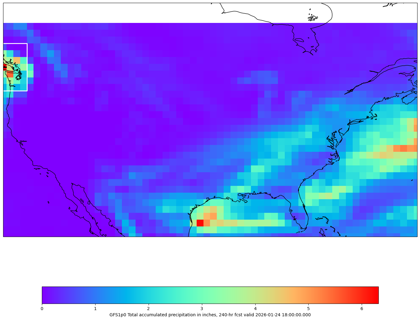

Create Region of Interest Image¶

Now crop the data and zoom in on the region of interest (ROI) to create a new plot.

# cmap = plt.get_cmap('rainbow')
fig, ax = make_map(bbox=roi_box)

cs = ax.pcolormesh(lons, lats, tp_inch, cmap=cmap)
cbar = fig.colorbar(cs, shrink=0.7, orientation='horizontal')
cbar.set_label(grid.getLocationName() + " Total accumulated precipitation in inches, " \
               + str(fcstHr) + "-hr fcst valid " + str(grid.getDataTime().getRefTime()))

ax.scatter(maxPoint.x, maxPoint.y, s=300,
           transform=ccrs.PlateCarree(),marker="+",facecolor='black')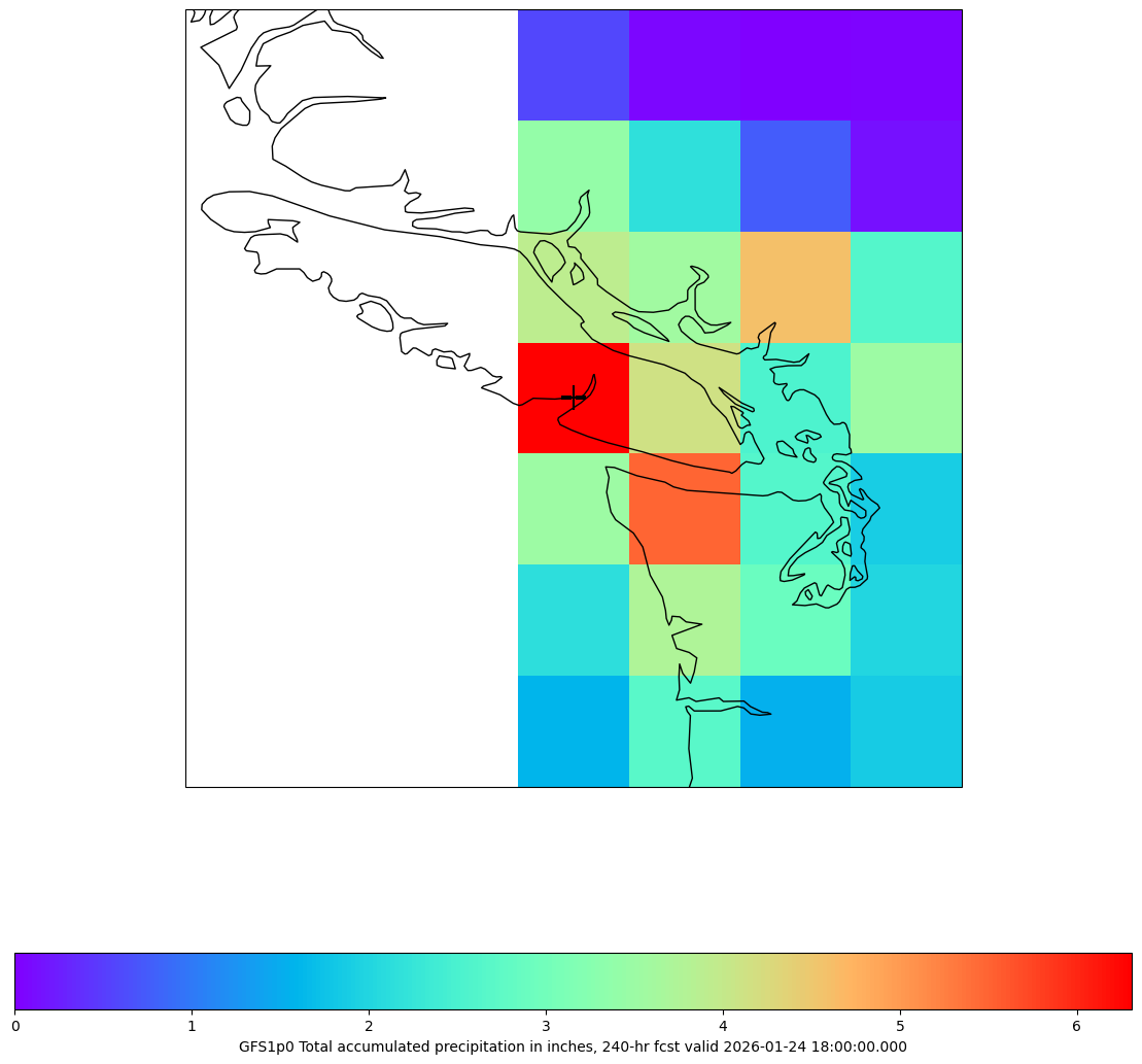

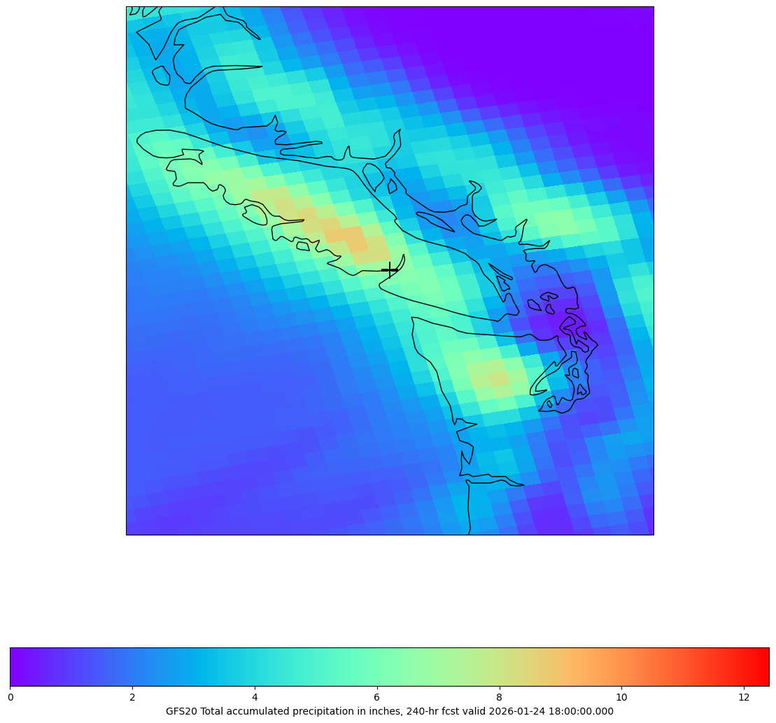
Top

High Resolution ROI¶

New Data Request¶

To see the region of interest more clearly, we can redo the process with a higher resolution model (GFS20 vs. GFS1.0).

roiRequest = DataAccessLayer.newDataRequest("grid", envelope=conus_envelope)
roiRequest.setLocationNames("GFS20")
roiRequest.setLevels("0.0SFC")
roiRequest.setParameters("TP")

roiCycles = DataAccessLayer.getAvailableTimes(roiRequest, True)
roiTimes = DataAccessLayer.getAvailableTimes(roiRequest)
roiFcstRun = DataAccessLayer.getForecastRun(roiCycles[-1], roiTimes)

Calculate Data¶

roiResponse = DataAccessLayer.getGridData(roiRequest, [roiFcstRun[-1]])  
print(roiResponse)
roiGrid = roiResponse[0]

roiLons, roiLats = roiGrid.getLatLonCoords()

roi_data, i, j = calculate_accumulated_precip(roiRequest, roiFcstRun)

roiFcstHr = int(roiGrid.getDataTime().getFcstTime()/3600)

[<awips.dataaccess.PyGridData.PyGridData object at 0x138a0ebd0>]

0.0 26.6875 3.0

0.0 55.125 6.0

0.0 66.625 9.0

0.0 67.8125 12.0

0.0 69.0625 15.0

0.0 71.6875 18.0

0.0 78.25 21.0

0.0 87.5 24.0

0.0 87.5 27.0

0.0 87.5 30.0

0.0 87.5625 33.0

0.0 87.5625 36.0

0.0 87.5625 39.0

0.0 87.5625 42.0

0.0 87.5625 45.0

0.0 87.5625 48.0

0.0 87.5625 51.0

0.0 87.5625 54.0

0.0 87.5625 57.0

0.0 87.5625 60.0

0.0 87.5625 63.0

0.0 87.5625 66.0

0.0 87.5625 69.0

0.0 87.5625 72.0

0.0 87.5625 75.0

0.0 87.5625 78.0

0.0 87.5625 81.0

0.0 87.5625 84.0

0.0 89.1875 90.0

0.0 91.0625 96.0

0.0 104.375 102.0

0.0 125.0625 108.0

0.0 137.9375 114.0

0.0 139.75 120.0

0.0 150.25 126.0

0.0 168.9375 132.0

0.0 217.4375 138.0

0.0 218.625 144.0

0.0 218.6875 150.0

0.0 218.6875 156.0

0.0 218.6875 162.0

0.0 218.6875 168.0

0.0 223.4375 174.0

0.0 232.5 180.0

0.0 250.8125 186.0

0.0 259.6875 192.0

0.0 262.3125 198.0

0.0 265.3125 204.0

0.0 282.4375 210.0

0.0 297.625 216.0

0.0 307.5625 222.0

0.0 313.4375 228.0

0.0 314.8125 234.0

0.0 315.375 240.0

Plot ROI¶

# cmap = plt.get_cmap('rainbow')
fig, ax = make_map(bbox=roi_box)

cs = ax.pcolormesh(roiLons, roiLats, roi_data, cmap=cmap)
cbar = fig.colorbar(cs, shrink=0.7, orientation='horizontal')
cbar.set_label(roiGrid.getLocationName() + " Total accumulated precipitation in inches, " \
               + str(roiFcstHr) + "-hr fcst valid " + str(roiGrid.getDataTime().getRefTime()))

ax.scatter(maxPoint.x, maxPoint.y, s=300,
           transform=ccrs.PlateCarree(),marker="+",facecolor='black')

Top

Precipitation Accumulation Region of Interest¶

Objectives¶

Table of Contents¶

Imports¶

Initial Setup¶

Geographic Filter¶

EDEX Connection¶

Refine the Request¶

Get Times¶

Function: calculate_accumulated_precip()¶

Fuction: make_map()¶

Get the Data!¶

Plot the Data!¶

Create CONUS Image¶

Create Region of Interest Image¶

High Resolution ROI¶

New Data Request¶

Calculate Data¶

Plot ROI¶

See Also¶

Additional Documentation¶

Precipitation Accumulation Region of Interest

Precipitation Accumulation Region of Interest¶

Objectives¶

Table of Contents¶

Imports¶

Initial Setup¶

Geographic Filter¶

EDEX Connection¶

Refine the Request¶

Get Times¶

Function: calculate_accumulated_precip()¶

Fuction: make_map()¶

Get the Data!¶

Plot the Data!¶

Create CONUS Image¶

Create Region of Interest Image¶

High Resolution ROI¶

New Data Request¶

Calculate Data¶

Plot ROI¶

See Also¶

Related Notebooks¶

Additional Documentation¶