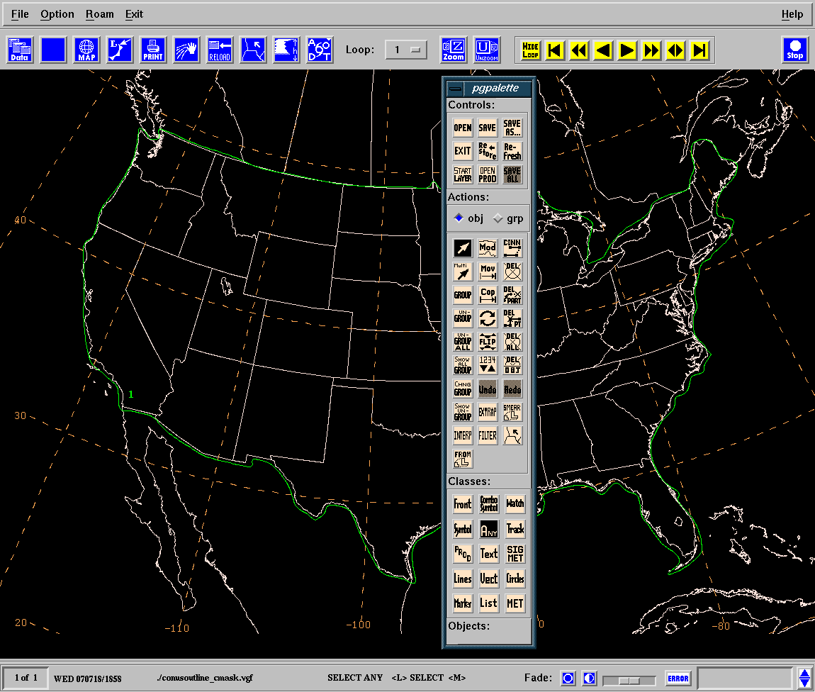
A vgf file is created using the interactive product generation tools within NMAP2. A closed line is drawn enclosing the region of interest, and a text label is grouped with the line assigning a value of 1 to the contour.

Once the region of interest is defined, a grid file can be created using the GRPHGD standalone program (It can also be created using the graph-to-grid option in NMAP2).
GEMPAK-GRPHGD>
GDOUTF   = 2007071900_cmask.grd
GUESS    =
PROJ     = MER
GRDAREA  =
KXKY     = 10;10
MAXGRD   = 200
CPYFIL   = #A218
ANLYSS   =
CNTRFL   = cmask.info
GDATTIM  = 070719/0000f000
GFUNC    = cmask
GLEVEL   = 0
GVCORD   = none
KEYCOL   =
KEYLINE  =
OLKDAY   =
GGLIMS   =
HISTGRD  = NO
BOUNDS   =
TYPE     = C
GAMMA    = 0.3
SEARCH   = 20
NPASS    = 2
QCNTL    =
GUESFUN  =
CATMAP   =
DISCRETE =
DLINES   = yes;no|-0.5
GGVGF    = conusoutline_cmask.vgf
EDGEOPTS =
GEMPAK-GRPHGD>r
GEMPAK-GDINFO>
GDFILE   = 2007071900_cmask.grd
LSTALL   = YES
OUTPUT   = T
GDATTIM  = all
GLEVEL   = 0
GVCORD   = none
GFUNC    = cmask
GEMPAK-GDINFO>r

GRID FILE: cmask.gem

GRID NAVIGATION:
    PROJECTION:          LCC
    ANGLES:                25.0   -95.0    25.0
    GRID SIZE:          614 428
    LL CORNER:              12.19   -133.46
    UR CORNER:              57.33    -49.42

Number of grids in file:     1

 NUM       TIME1              TIME2           LEVL1 LEVL2  VCORD PARM
   1     070719/0000F000                          0         NONE CMASK
GEMPAK-GDINFO>
The parameter CMASK is created where values greater than 1 are enclosed by the contour. DLINES defines the epsilon of (here -0.5 is used since the contour was drawn counterclockwise) to add to vlaues on either side of the single contour to be define greater / less than the contour value of 1.0.
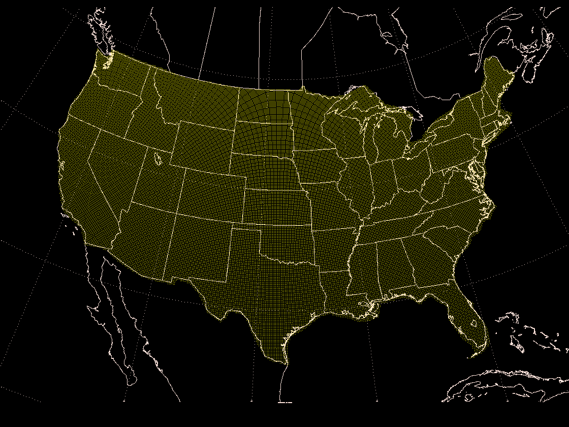
The grid point values of SGT(cmask,1) (greater than 1.0) as shown here:
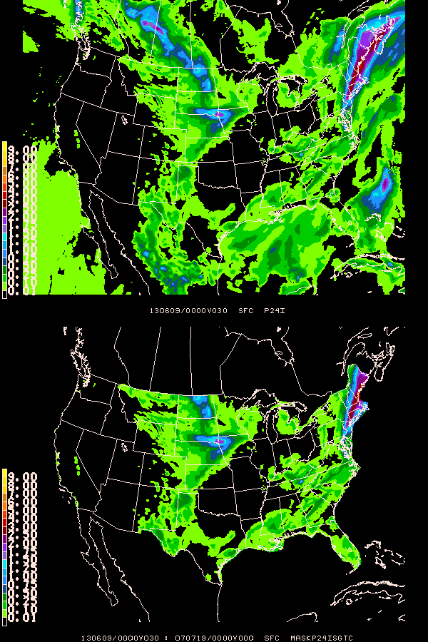
The resultant grid can ge used with the MASK() function and logical operators to define mask or clipping regions of interest. As an example, the 24 hour precipitation in the top panel is masked by the region of interest in the lower panel so that only data within the region of interest will be considered.
GDFILE  = nam12 + 2007071900_cmask.grd
GDATTIM  = f030
GLEVEL   = 0
GVCORD   = none
PANEL    = t     ! b
SKIP     = 0
SCALE    = 0
GDPFUN   = p24i  ! mask(p24i,sgt(cmask^070719/0000f000+2,1))
TYPE     = f
CONTUR   = 3/3
CINT     = 0
LINE     = 2/1/2
FINT     = .01;.1;.25;.5;.75;1;1.25;1.5;1.75;2;2.5;3;4;5;6;7;8;9
FLINE    = 0;21-30;14-20;5
HILO     =
HLSYM    =
CLRBAR   = 1
WIND     = BM1
REFVEC   =
TITLE    = 1
TEXT     = 0.7/2/SW
CLEAR    = YES
GAREA    = us
IJSKIP   =
PROJ     = STR/90;-100;0
The HIGH() function can be used to obtain local maximas from the grid region of interest. The GWFS() gaussian weighted smoothing function can be used to reduce higher frequency features in the grid and focus on broader areas of interest. By using the GDCSV program, the locations of HIGH() output are output to a file for use in determining local mesoscale model domain centers. By masking the region, the model domains are ensured to be within the desired region.
GEMPAK-GDCSV>l
GDATTIM  = f030
GDFILE   = nam12 + 2007071900_cmask.grd
GLEVEL   = 0
GAREA    = grid
PROJ     = def
GVCORD   = none
GFUNC    = high(mask(gwfs(p24i,40),sgt(cmask^070719/0000f000+2,1)),30)
SCALE    = 0
OUTPUT   = f/p24i_highs.dat
GEMPAK-GDCSV>r
OUTPUT is to the text file p24i_highs.dat. You can use the sort command to return the top two local maxima:
sort -t, -k 5bnr p24i_highs.dat | head -2

 508,     244,        42.3889,       -72.2385,        2.53370
 338,     236,        42.9560,       -96.3721,        0.58850
These two values are now scriptable (use |head -1 for the first and
| head -2 | tail -1 for the second) both for plotting regional areas of
interest and for WRF domains.
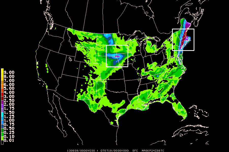
The locations of the 2 greatest local maximas (42.3889,-72.2385 and 42.9560,-96.3721) are shown along with the precipitation forecast field. The primary and secondary domains can be drawn using GPANOT to overlay the boxes.
First plot masked precipitation, same as above, but change PANEL = 0 and CLEAR = n
GDFILE   = nam12 + 2007071900_cmask.grd
GDATTIM  = f030
GLEVEL   = 0
GVCORD   = none
PANEL    = 0
SKIP     = 0
SCALE    = 0
GDPFUN   = mask(p24i,sgt(cmask^070719/0000f000+2,1))
TYPE     = f
CONTUR   = 3/3
CINT     = 0
LINE     = 2/1/2
FINT     = .01;.1;.25;.5;.75;1;1.25;1.5;1.75;2;2.5;3;4;5;6;7;8;9
FLINE    = 0;21-30;14-20;5
HILO     =
HLSYM    =
CLRBAR   = 1
WIND     = BM1
REFVEC   =
TITLE    = 1
TEXT     = 0.7/2/SW
CLEAR    = YES
GAREA    = us
IJSKIP   =
PROJ     = STR/90;-100;0
CLEAR    = n
r
