xarray with MetPy Tutorial

xarray is a powerful Python package that provides N-dimensional labeled arrays and datasets following the Common Data Model. While the process of integrating xarray features into MetPy is ongoing, this tutorial demonstrates how xarray can be used within the current version of MetPy. MetPy’s integration primarily works through accessors which allow simplified projection handling and coordinate identification. Unit and calculation support is currently available in a limited fashion, but should be improved in future versions.

import cartopy.crs as ccrs
import cartopy.feature as cfeature
import matplotlib.pyplot as plt
import xarray as xr

# Any import of metpy will activate the accessors
import metpy.calc as mpcalc
from metpy.cbook import get_test_data
from metpy.units import units

Getting Data

While xarray can handle a wide variety of n-dimensional data (essentially anything that can be stored in a netCDF file), a common use case is working with model output. Such model data can be obtained from a THREDDS Data Server using the siphon package, but for this tutorial, we will use an example subset of GFS data from Hurrican Irma (September 5th, 2017).

# Open the netCDF file as a xarray Dataset
data = xr.open_dataset(get_test_data('irma_gfs_example.nc', False))

# View a summary of the Dataset
print(data)

Out:

<xarray.Dataset>
Dimensions:                              (isobaric1: 21, isobaric3: 31, latitude: 81, longitude: 131, time1: 9)
Coordinates:
  * time1                                (time1) datetime64[ns] 2017-09-05T12...
    reftime                              datetime64[ns] ...
  * latitude                             (latitude) float32 50.0 49.5 ... 10.0
  * isobaric3                            (isobaric3) float64 100.0 ... 1e+05
  * isobaric1                            (isobaric1) float64 1e+04 ... 1e+05
  * longitude                            (longitude) float32 250.0 ... 315.0
Data variables:
    Vertical_velocity_pressure_isobaric  (time1, isobaric1, latitude, longitude) float32 ...
    Relative_humidity_isobaric           (time1, isobaric3, latitude, longitude) float32 ...
    Temperature_isobaric                 (time1, isobaric3, latitude, longitude) float32 ...
    u-component_of_wind_isobaric         (time1, isobaric3, latitude, longitude) float32 ...
    v-component_of_wind_isobaric         (time1, isobaric3, latitude, longitude) float32 ...
    Geopotential_height_isobaric         (time1, isobaric3, latitude, longitude) float32 ...
    LatLon_361X720-0p25S-180p00E         int32 ...
Attributes:
    Originating_or_generating_Center:                                        ...
    Originating_or_generating_Subcenter:                                     ...
    GRIB_table_version:                                                      ...
    Type_of_generating_process:                                              ...
    Analysis_or_forecast_generating_process_identifier_defined_by_originating...
    Conventions:                                                             ...
    history:                                                                 ...
    featureType:                                                             ...
    History:                                                                 ...
    geospatial_lat_min:                                                      ...
    geospatial_lat_max:                                                      ...
    geospatial_lon_min:                                                      ...
    geospatial_lon_max:                                                      ...

Preparing Data

To make use of the data within MetPy, we need to parse the dataset for projection information following the CF conventions. For this, we use the data.metpy.parse_cf() method, which will return a new, parsed DataArray or Dataset.

Additionally, we rename our data variables for easier reference.

# To parse the full dataset, we can call parse_cf without an argument, and assign the returned
# Dataset.
data = data.metpy.parse_cf()

# If we instead want just a single variable, we can pass that variable name to parse_cf and
# it will return just that data variable as a DataArray.
data_var = data.metpy.parse_cf('Temperature_isobaric')

# If we want only a subset of variables, we can pass a list of variable names as well.
data_subset = data.metpy.parse_cf(['u-component_of_wind_isobaric',
                                   'v-component_of_wind_isobaric'])

# To rename variables, supply a dictionary between old and new names to the rename method
data = data.rename({
    'Vertical_velocity_pressure_isobaric': 'omega',
    'Relative_humidity_isobaric': 'relative_humidity',
    'Temperature_isobaric': 'temperature',
    'u-component_of_wind_isobaric': 'u',
    'v-component_of_wind_isobaric': 'v',
    'Geopotential_height_isobaric': 'height'
})

Units

MetPy’s DataArray accessor has a unit_array property to obtain a pint.Quantity array of just the data from the DataArray (metadata other than units is removed) and a convert_units method to convert the the data from one unit to another (keeping it as a DataArray). For now, we’ll just use convert_units to convert our temperature to degC.

data['temperature'].metpy.convert_units('degC')

WARNING: Versions of MetPy prior to 1.0 (including 0.12) require units to be in the attributes of your xarray DataArray. If you attempt to use a DataArray containing a pint.Quantity instead, incorrect results are likely to occur, since these earlier versions of MetPy will ignore the pint.Quantity and still just rely upon the units attribute. See GitHub Issue #1358 for more details.

Note that this changes in newer versions of MetPy as of 1.0, when Quantities-in-xarray became the default behavior.

Coordinates

You may have noticed how we directly accessed the vertical coordinates above using their names. However, in general, if we are working with a particular DataArray, we don’t have to worry about that since MetPy is able to parse the coordinates and so obtain a particular coordinate type directly. There are two ways to do this:

1. Use the data_var.metpy.coordinates method

2. Use the data_var.metpy.x, data_var.metpy.y, data_var.metpy.longitude, data_var.metpy.latitude, data_var.metpy.vertical, data_var.metpy.time properties

The valid coordinate types are:

• x

• y

• longitude

• latitude

• vertical

• time

(Both approaches are shown below)

The x, y, vertical, and time coordinates cannot be multidimensional, however, the longitude and latitude coordinates can (which is often the case for gridded weather data in its native projection). Note that for gridded data on an equirectangular projection, such as the GFS data in this example, x and longitude will be identical (as will y and latitude).

# Get multiple coordinates (for example, in just the x and y direction)
x, y = data['temperature'].metpy.coordinates('x', 'y')

# If we want to get just a single coordinate from the coordinates method, we have to use
# tuple unpacking because the coordinates method returns a generator
vertical, = data['temperature'].metpy.coordinates('vertical')

# Or, we can just get a coordinate from the property
time = data['temperature'].metpy.time

# To verify, we can inspect all their names
print([coord.name for coord in (x, y, vertical, time)])

Out:

['longitude', 'latitude', 'isobaric3', 'time1']

Indexing and Selecting Data

MetPy provides wrappers for the usual xarray indexing and selection routines that can handle quantities with units. For DataArrays, MetPy also allows using the coordinate axis types mentioned above as aliases for the coordinates. And so, if we wanted 850 hPa heights, we would take:

print(data['height'].metpy.sel(vertical=850 * units.hPa))

Out:

<xarray.DataArray 'height' (time1: 9, latitude: 81, longitude: 131)>
array([[[1593.8025, 1594.1064, ..., 1453.2264, 1458.3625],
        [1594.7784, 1595.0825, ..., 1463.3065, 1468.4905],
        ...,
        [1511.4985, 1511.8025, ..., 1537.6584, 1536.9385],
        [1511.2745, 1511.9305, ..., 1537.9146, 1537.0825]],

       [[1590.0658, 1590.8018, ..., 1463.2977, 1465.3617],
        [1591.5537, 1591.9377, ..., 1472.6577, 1475.2338],
        ...,
        [1522.8977, 1523.2977, ..., 1536.4337, 1535.5857],
        [1523.0417, 1523.4738, ..., 1536.7058, 1535.6978]],

       ...,

       [[1546.7413, 1547.8773, ..., 1553.7174, 1555.9254],
        [1547.8453, 1549.2374, ..., 1563.6373, 1565.6533],
        ...,
        [1514.6774, 1514.1814, ..., 1524.7733, 1524.3093],
        [1515.4934, 1515.0294, ..., 1524.8214, 1524.3414]],

       [[1542.1625, 1542.6906, ..., 1561.7946, 1564.2264],
        [1542.2426, 1543.2345, ..., 1571.6665, 1574.0825],
        ...,
        [1507.6505, 1507.2025, ..., 1538.3385, 1537.8905],
        [1508.5625, 1508.0505, ..., 1538.8185, 1538.6105]]], dtype=float32)
Coordinates:
  * time1      (time1) datetime64[ns] 2017-09-05T12:00:00 ... 2017-09-06T12:0...
    reftime    datetime64[ns] 2017-09-05T12:00:00
  * latitude   (latitude) float32 50.0 49.5 49.0 48.5 ... 11.5 11.0 10.5 10.0
  * longitude  (longitude) float32 250.0 250.5 251.0 251.5 ... 314.0 314.5 315.0
    crs        object Projection: latitude_longitude
    isobaric3  float64 8.5e+04
Attributes:
    long_name:                      Geopotential height @ Isobaric surface
    units:                          gpm
    Grib_Variable_Id:               VAR_0-3-5_L100
    Grib2_Parameter:                [0 3 5]
    Grib2_Parameter_Discipline:     Meteorological products
    Grib2_Parameter_Category:       Mass
    Grib2_Parameter_Name:           Geopotential height
    Grib2_Level_Type:               100
    Grib2_Level_Desc:               Isobaric surface
    Grib2_Generating_Process_Type:  Forecast
    grid_mapping:                   LatLon_361X720-0p25S-180p00E

For full details on xarray indexing/selection, see xarray’s documentation.

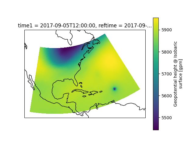
Projections

Getting the cartopy coordinate reference system (CRS) of the projection of a DataArray is as straightforward as using the data_var.metpy.cartopy_crs property:

data_crs = data['temperature'].metpy.cartopy_crs
print(data_crs)

Out:

<cartopy.crs.PlateCarree object at 0x7fa25c152230>

The cartopy Globe can similarly be accessed via the data_var.metpy.cartopy_globe property:

data_globe = data['temperature'].metpy.cartopy_globe
print(data_globe)

Out:

<cartopy._crs.Globe object at 0x7fa2714bd210>

Calculations

Most of the calculations in metpy.calc will accept DataArrays by converting them into their corresponding unit arrays. While this may often work without any issues, we must keep in mind that because the calculations are working with unit arrays and not DataArrays:

• The calculations will return unit arrays rather than DataArrays

• Broadcasting must be taken care of outside of the calculation, as it would only recognize dimensions by order, not name

As an example, we calculate geostropic wind at 500 hPa below:

lat, lon = xr.broadcast(y, x)
f = mpcalc.coriolis_parameter(lat)
dx, dy = mpcalc.lat_lon_grid_deltas(lon, lat, initstring=data_crs.proj4_init)
heights = data['height'].metpy.loc[{'time': time[0], 'vertical': 500. * units.hPa}]
u_geo, v_geo = mpcalc.geostrophic_wind(heights, f, dx, dy)
print(u_geo)
print(v_geo)

Out:

[[2.2725555398031156 6.251403116857854 3.2825541563237786 ...  33.11408008114585 32.73451716892398 32.5765366055535] [3.816296728549826 4.388776144480824 4.325234764565967 ...  31.008031569492147 30.753751181686432 30.53090851162976] [5.127333709607048 4.839104240493513 5.800602961394321 ...  29.193825139174717 29.033832384148585 28.58473285322843] ... [-1.9117831398732483 -1.1464325905754669 -1.91181664555917 ...  -7.0079228001080995 -7.392149528166841 -6.88190745221371] [-2.8016460018049023 -2.6697320073045367 -2.4025371858986984 ...  -6.404532768301047 -7.204303662756457 -6.93719274537382] [-7.13845125502525 -8.405095361594876 -3.6393431096920725 ...  -5.606968107542709 -7.557393778305965 -8.398398522461456]] meter / second
[[-14.791524808043887 -14.39816816884509 -16.89520567938152 ...  5.582914366984641 6.513698998038233 7.396061307243545] [-8.301012127894664 -13.770643557272367 -17.09080997637208 ...  5.273521060998235 6.103860705847083 7.179189291138215] [-11.98245046368792 -13.54015713307823 -14.854695089573378 ...  4.919261443711342 5.7474619744198705 6.721325915052195] ... [4.25739861885645 3.4827536038902918 2.966323593912038 ...  3.224538598899942 3.2245385989023876 1.9334635739628656] [6.609707782452212 3.1007692883802775 2.0210959055875346 ...  2.4259734241357735 3.63896013620366 3.3723334776431315] [4.799363905563508 4.2371674868632 2.5436801152315818 ...  1.5555250602976798 2.9679142225845174 3.812933379494143]] meter / second

Also, a limited number of calculations directly support xarray DataArrays or Datasets (they can accept and return xarray objects). Right now, this includes

• Derivative functions

  • first_derivative

  • second_derivative

  • gradient

  • laplacian

• Cross-section functions

  • cross_section_components

  • normal_component

  • tangential_component

  • absolute_momentum

More details can be found by looking at the documentation for the specific function of interest.

There is also the special case of the helper function, grid_deltas_from_dataarray, which takes a DataArray input, but returns unit arrays for use in other calculations. We could rewrite the above geostrophic wind example using this helper function as follows:

heights = data['height'].metpy.loc[{'time': time[0], 'vertical': 500. * units.hPa}]
lat, lon = xr.broadcast(y, x)
f = mpcalc.coriolis_parameter(lat)
dx, dy = mpcalc.grid_deltas_from_dataarray(heights)
u_geo, v_geo = mpcalc.geostrophic_wind(heights, f, dx, dy)
print(u_geo)
print(v_geo)

Out:

[[2.2725555398031156 6.251403116857854 3.2825541563237786 ...  33.11408008114585 32.73451716892398 32.5765366055535] [3.816296728549826 4.388776144480824 4.325234764565967 ...  31.008031569492147 30.753751181686432 30.53090851162976] [5.127333709607048 4.839104240493513 5.800602961394321 ...  29.193825139174717 29.033832384148585 28.58473285322843] ... [-1.9117831398732483 -1.1464325905754669 -1.91181664555917 ...  -7.0079228001080995 -7.392149528166841 -6.88190745221371] [-2.8016460018049023 -2.6697320073045367 -2.4025371858986984 ...  -6.404532768301047 -7.204303662756457 -6.93719274537382] [-7.13845125502525 -8.405095361594876 -3.6393431096920725 ...  -5.606968107542709 -7.557393778305965 -8.398398522461456]] meter / second
[[-14.791524808043887 -14.39816816884509 -16.89520567938152 ...  5.582914366984641 6.513698998038233 7.396061307243545] [-8.301012127894664 -13.770643557272367 -17.09080997637208 ...  5.273521060998235 6.103860705847083 7.179189291138215] [-11.98245046368792 -13.54015713307823 -14.854695089573378 ...  4.919261443711342 5.7474619744198705 6.721325915052195] ... [4.25739861885645 3.4827536038902918 2.966323593912038 ...  3.224538598899942 3.2245385989023876 1.9334635739628656] [6.609707782452212 3.1007692883802775 2.0210959055875346 ...  2.4259734241357735 3.63896013620366 3.3723334776431315] [4.799363905563508 4.2371674868632 2.5436801152315818 ...  1.5555250602976798 2.9679142225845174 3.812933379494143]] meter / second

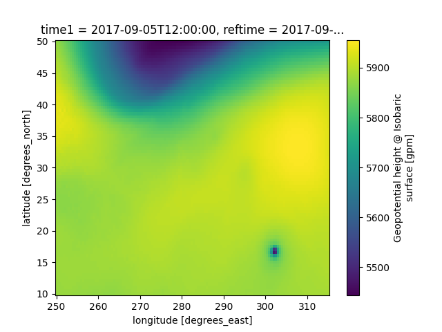
Plotting

Like most meteorological data, we want to be able to plot these data. DataArrays can be used like normal numpy arrays in plotting code, which is the recommended process at the current point in time, or we can use some of xarray’s plotting functionality for quick inspection of the data.

(More detail beyond the following can be found at xarray’s plotting reference.)

# A very simple example example of a plot of 500 hPa heights
data['height'].metpy.loc[{'time': time[0], 'vertical': 500. * units.hPa}].plot()
plt.show()

# Let's add a projection and coastlines to it
ax = plt.axes(projection=ccrs.LambertConformal())
data['height'].metpy.loc[{'time': time[0],
                          'vertical': 500. * units.hPa}].plot(ax=ax, transform=data_crs)
ax.coastlines()
plt.show()

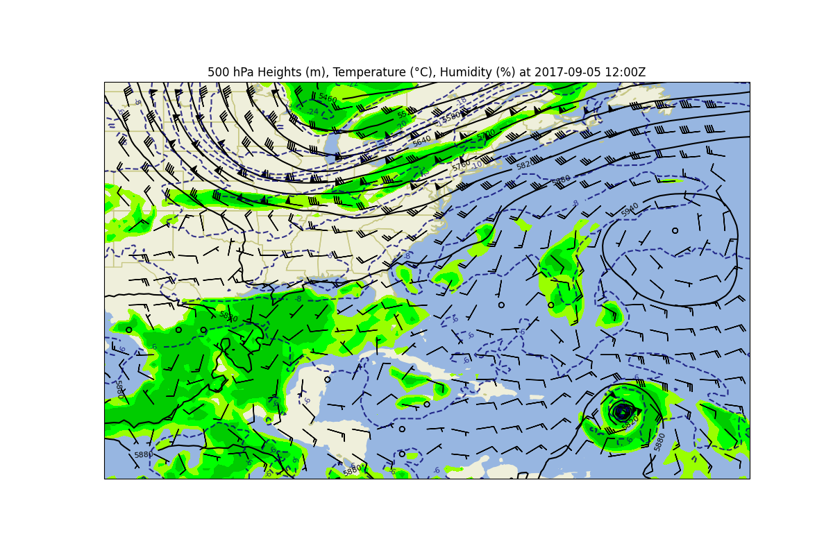
# Or, let's make a full 500 hPa map with heights, temperature, winds, and humidity

# Select the data for this time and level
data_level = data.metpy.loc[{time.name: time[0], vertical.name: 500. * units.hPa}]

# Create the matplotlib figure and axis
fig, ax = plt.subplots(1, 1, figsize=(12, 8), subplot_kw={'projection': data_crs})

# Plot RH as filled contours
rh = ax.contourf(x, y, data_level['relative_humidity'], levels=[70, 80, 90, 100],
                 colors=['#99ff00', '#00ff00', '#00cc00'])

# Plot wind barbs, but not all of them
wind_slice = slice(5, -5, 5)
ax.barbs(x[wind_slice], y[wind_slice],
         data_level['u'].metpy.unit_array[wind_slice, wind_slice].to('knots'),
         data_level['v'].metpy.unit_array[wind_slice, wind_slice].to('knots'),
         length=6)

# Plot heights and temperature as contours
h_contour = ax.contour(x, y, data_level['height'], colors='k', levels=range(5400, 6000, 60))
h_contour.clabel(fontsize=8, colors='k', inline=1, inline_spacing=8,
                 fmt='%i', rightside_up=True, use_clabeltext=True)
t_contour = ax.contour(x, y, data_level['temperature'], colors='xkcd:deep blue',
                       levels=range(-26, 4, 2), alpha=0.8, linestyles='--')
t_contour.clabel(fontsize=8, colors='xkcd:deep blue', inline=1, inline_spacing=8,
                 fmt='%i', rightside_up=True, use_clabeltext=True)

# Add geographic features
ax.add_feature(cfeature.LAND.with_scale('50m'), facecolor=cfeature.COLORS['land'])
ax.add_feature(cfeature.OCEAN.with_scale('50m'), facecolor=cfeature.COLORS['water'])
ax.add_feature(cfeature.STATES.with_scale('50m'), edgecolor='#c7c783', zorder=0)
ax.add_feature(cfeature.LAKES.with_scale('50m'), facecolor=cfeature.COLORS['water'],
               edgecolor='#c7c783', zorder=0)

# Set a title and show the plot
ax.set_title('500 hPa Heights (m), Temperature (\u00B0C), Humidity (%) at '
             + time[0].dt.strftime('%Y-%m-%d %H:%MZ').item())
plt.show()

What Could Go Wrong?

Depending on your dataset and what you are trying to do, you might run into problems with xarray and MetPy. Below are examples of some of the most common issues

• Multiple coordinate conflict

• An axis not being available

• An axis not being interpretable

• Arrays not broadcasting in calculations

Coordinate Conflict

Code:

x = data['Temperature'].metpy.x

Error Message:

/home/user/env/MetPy/metpy/xarray.py:305: UserWarning: More than
one x coordinate present for variable "Temperature".

Fix:

Manually assign the coordinates using the assign_coordinates() method on your DataArray, or by specifying the coordinates argument to the parse_cf() method on your Dataset, to map the time, vertical, y, latitude, x, and longitude axes (as applicable to your data) to the corresponding coordinates.

data['Temperature'].assign_coordinates({'time': 'time', 'vertical': 'isobaric',
                                        'y': 'y', 'x': 'x'})
x = data['Temperature'].metpy.x

or

temperature = data.metpy.parse_cf('Temperature',
                                  coordinates={'time': 'time', 'vertical': 'isobaric',
                                               'y': 'y', 'x': 'x'})
x = temperature.metpy.x

Axis Unavailable

Code:

data['Temperature'].metpy.vertical

Error Message:

AttributeError: vertical attribute is not available.

This means that your data variable does not have the coordinate that was requested, at least as far as the parser can recognize. Verify that you are requesting a coordinate that your data actually has, and if it still is not available, you will need to manually specify the coordinates as discussed above.

Axis Not Interpretable

Code:

x, y, ensemble = data['Temperature'].metpy.coordinates('x', 'y', 'ensemble')

Error Message:

AttributeError: 'ensemble' is not an interpretable axis

This means that you are requesting a coordinate that MetPy is (currently) unable to parse. While this means it cannot be recognized automatically, you can still obtain your desired coordinate directly by accessing it by name. If you have a need for systematic identification of a new coordinate type, we welcome pull requests for such new functionality on GitHub!

Broadcasting in Calculations

Code:

theta = mpcalc.potential_temperature(data['isobaric3'], data['temperature'])

Error Message:

ValueError: operands could not be broadcast together with shapes (9,31,81,131) (31,)

This is a symptom of the incomplete integration of xarray with MetPy’s calculations; the calculations currently convert the DataArrays to unit arrays that do not recognize which coordinates match with which. And so, we must do some manipulations.

Fix 1 (xarray broadcasting):

pressure, temperature = xr.broadcast(data['isobaric3'], data['temperature'])
theta = mpcalc.potential_temperature(pressure, temperature)

Fix 2 (unit array broadcasting):

theta = mpcalc.potential_temperature(
    data['isobaric3'].metpy.unit_array[None, :, None, None],
    data['temperature'].metpy.unit_array
)