%matplotlib inline

# Copyright (c) 2023 MetPy Developers.
# Distributed under the terms of the BSD 3-Clause License.
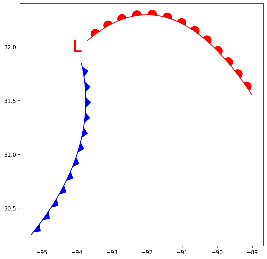
# SPDX-License-Identifier: BSD-3-Clause

Simple Plotting of Fronts¶

This uses MetPy’s path effects for matplotlib that can be used to represent a line as a traditional front. This example relies on already having location information for the boundaries you would like to plot.

import matplotlib.pyplot as plt
import numpy as np

from metpy.plots import ColdFront, WarmFront

Define some synthetic points to represent the low pressure system and its frontal boundaries.

low_lon, low_lat = -94, 32
cold_lat = np.linspace(low_lat - 0.15, low_lat - 1.75, 100)
cold_lon = (low_lon + 0.25) - (cold_lat - (low_lat - 0.5))**2

warm_lon = np.linspace(low_lon + 0.3, low_lon + 5, 100)
warm_lat = (low_lat + 0.3) - (warm_lon - (low_lon + 2))**2 / 12

Draw the low as an “L” using matplotlib’s text() method, then plot the fronts as standard lines, but add our path effects.

fig, ax = plt.subplots(figsize=(8, 8), dpi=150)
ax.text(low_lon, low_lat, 'L', color='red', size=30,
        horizontalalignment='center', verticalalignment='center')
ax.plot(cold_lon, cold_lat, 'blue', path_effects=[ColdFront(size=8, spacing=1.5)])
ax.plot(warm_lon, warm_lat, 'red', path_effects=[WarmFront(size=8, spacing=1.5)])
plt.show()